Coordinate Systems
3D coordinate systems are used to describe the position and orientation of objects in space. While CityEngine can handle many different types of (georeferenced) coordinate systems, CGA modeling works with Cartesian coordinate systems only. A coordinate system is defined by its origin and the orientation of the three orthogonal axis. While one global coordinate system would be sufficient to define each vertex of a geometry, it is more practical to use a hierarchy of coordinate systems that are defined relative to each other.
Think of a car model placed on a street segment. It makes sense to define the position of the wheels relative to the car and the car relative to the street. The origin and the orientation of the "car" system are defined with coordinates of the "street" system. This way the two coordinate systems are relative to each other and the coordinates of one system can be translated into coordinates of the other one.
Several coordinate systems are involved when working with shapes. All transformations described above operate in the system defined by the current shape's scope, the scope system. There is also a pivot system associated to each shape, and every shape defines an object coordinate system.
There are multiple different coordinate systems relative to each other in CGA:
World Coordinate System 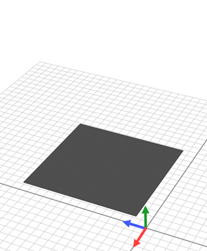 |
|
Object Coordinate System 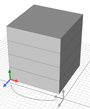 |
|
Pivot Coordinate System 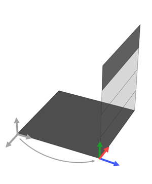 |
|
Scope Coordinate System 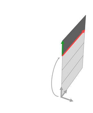 |
|
Note:
- When developing CGA rules you can visualise the coordinate systems and shapes of a model using the Model Heirarchy.
- You can query the pivot and scope attribute attributes.
CGA shapes
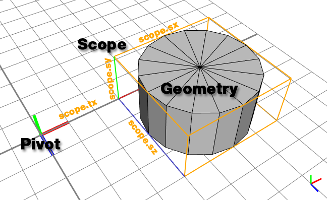
CGA Shapes are the central ingredient of the CGA shape grammar. A Shape consists of a geometry in an oriented bounding box, the scope . The scope is placed relative to the pivot.
Note:
Initial shapes serve as a starting CGA shape for CGA rules, see Shapes
A Shape has the following components:
Shape Symbol | The name of the shape. Used to find the matching rule that is used to generate the successive shapes. |
Pivot | The pivot describes the shape's coordinate system and is defined by:
The pivot is given in object coordinates, relative to the initial shape's origin; see Coordinate Systems. |
Scope | The scope represents the oriented bounding box for the shape in space relative to the pivot and is defined by three vectors:
|
Geometry | The geometry contains the information about the corners edges and faces that make up the "form" of the shape. The geometry can be any sort of polygonal mesh. In addition, information about color, material and textures (shader attributes) are stored in the geometry as well. |
Parameters | Each shape can have an associated parameter list. The ordered parameter list is implicitly defined in the rule which creates the shape. Three parameter types are supported:
|
Rule application
The basic idea of a rule is to replace a shape with a certain shape symbol with a number of new shapes. Formally:
PredecessorShape --> Successor
Here is a simple example:
A --> B
On application on a specific shape with symbol A, the rule above creates a copy of the shape and sets its shape symbol to B. The A shape is now considered done and not processed anymore. If there is no rule matching symbol B the generation process is finished. The resulting structure is called the shape tree and looks like this:

In the shape tree above, A is the root shape and B is a leaf shape. Leaves are very important because the sum of all leaves represents the generated model. Inner nodes are not visible in the final model.
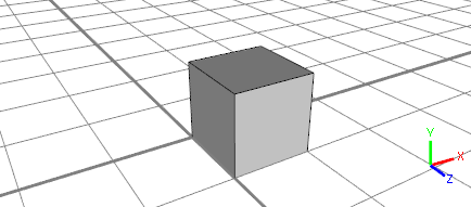
In this simple example, we assume shape A's geometry, scope and pivot are set up such that the shape represents a unit cube in the origin; because B is a copy of A, B looks exactly the same (see the picture above).
A rule can have more complex successors, e.g., the right side of the rule can consist of multiple shape symbols and shape operations:
A --> B t(3, 0, 0) C
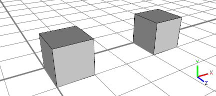
This successor is now executed from the left to the right. Again, B is an identical copy of A. Then the current shape is translated by 3 units in x-direction (i.e., the scope.t is manipulated) and a new shape C is created. The shape tree now has two leaves:
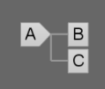
The two leaves B and C make up the final 3D model:
If we add this rule for C:
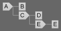
C --> D s(2, 0.5, 1.75) E
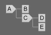
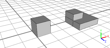
The generation process will add two children, D and E to shape C. Shape D is an exact copy of shape C, but shape E will have a different sized scope (because of the s() shape operation). The shape tree and the associated model look like this:
Note:
Now, the leaves (B, D, E) are not on the same level (i.e. have different distances to the root shape) but they are all part of the model.
Another shape operation is the insert operation i():
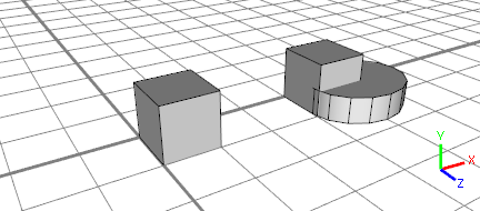
E --> i("cylinder.obj") F
After starting the generation again, shape E is not a leaf anymore but now has a child shape F.
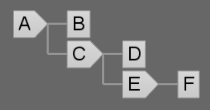
The geometry of shape F is not a cube anymore but was replaced with the mesh read from file "cylinder.obj".
Note:
The size (i.e. the scope.s vector) of shape F is still the same as the one of shape E.
Terminal Shapes
In the E rule above, F is a so-called terminal shape: because no rule F is defined, the generation is stopped at this point. However, the CGA editor will issue a "Undefined Rule" warning. This can be suppressed by adding a period after F, thus explicitly marking F as a terminal shape:
E --> i("cylinder.obj") F.
Anonymous Leaf Shapes
For convenience, rules like the E rule above can be truncated:
E --> i("cylinder.obj")
In this case (i.e. E has no children), the rule interpreter silently inserts an anonymous leaf with the same name as the rule itself. The shape tree after applying the E rule above looks like this:
