Seasonal-Trend decomposition using LOESS

Seasonal-Trend decomposition using LOESS (STL) is a robust method of time series decomposition often used in economic and environmental analyses. The STL method uses locally fitted regression models to decompose a time series into trend, seasonal, and remainder components.

About STL

You can apply STL to any dataset, but meaningful results are only returned if a recurring temporal pattern exists in the data (for example, air quality decreasing during warmer months or online shopping increasing in the fourth quarter of every year). The pattern is displayed in the STL results as the seasonal component.

The STL algorithm performs smoothing on the time series using LOESS in two loops; the inner loop iterates between seasonal and trend smoothing and the outer loop minimizes the effect of outliers. During the inner loop, the seasonal component is calculated first and removed to calculate the trend component. The remainder is calculated by subtracting the seasonal and trend components from the time series.

The three components of STL analysis relate to the raw time series as follows:

yi = si + ti + ri

where:

• y_i = The value of the time series at point i.
• s_i = The value of the seasonal component at point i.
• t_i = The value of the trend component at point i.
• r_i = The value of the remainder component at point i.

Examples

A meteorologist is studying the effect of climate change on the frequency of tornados in the United States. She uses STL to decompose a time series of tornado counts to determine how seasonality affects the frequency of tornados and whether the frequency of tornados increased over time. The meteorologist can then compare the trends in tornados to other climate trends, such as mean global temperature, to determine if climate change is a factor in increasing frequency of tornados.

An economist is tracking gas prices in his region and looking for overall trends in prices over time. He knows that gas prices tend to increase in summer months, so he uses STL analysis to decompose the time series of gas prices and analyze the trend separately from the seasonal component.

Seasonal component

The seasonal component of an STL output shows the recurring temporal pattern present in the data based on the chosen seasonality. If a seasonal pattern exists, it normally takes the shape of an oscillating or wave pattern.

Smoothing for the seasonal component is performed for each subseries (week, month, quarter, or year) separately. For example, if using STL with monthly seasonality on a dataset with data collected daily from January 2015 to December 2020, the smoothing is performed first on all data collected in January for all years, then February for all years, and so on until all months have had smoothing performed. The subseries are then recombined to create the seasonal component.

Example

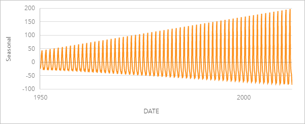
The following example shows the seasonal component of an STL analysis using tornado incidents across the United States. The component was calculated using monthly seasonality and oscillates between a high count in June and a low count in January. The oscillations increase in amplitude over time, which indicates that the seasonal variation in tornado frequency is increasing over time.

Trend component

The trend component is the second component calculated during the inner loop. The values for the seasonal component are subtracted from the raw data, eliminating seasonal variation from the time series. A smoothed trend line is then created by applying LOESS to the remaining values.

Example

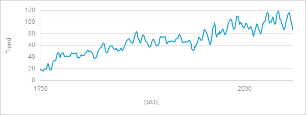
The following example shows the trend component of an STL analysis using tornado incidents across the United States. The result shows an overall positive trend, meaning that the number of tornado incidents in the United States is increasing over time.

Remainder component

The remainder component is calculated by subtracting the values of the seasonal and trend component from the time series. Remainder values indicate the amount of noise present in the data. Values close to zero indicate that the seasonal and trend components are accurate in describing the time series, whereas larger remainder values indicate the presence of noise.

You can also use the remainder component to identify outliers in the data, which appear as relatively large positive or negative values compared to the other remainder values.

Example

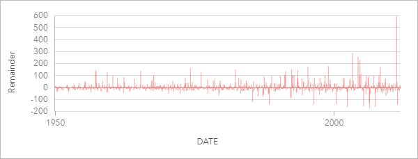
The following example shows the remainder component of an STL analysis using tornado incidents across the United States. The remainder values begin relatively small and become larger in later years, which indicates that the amount of noise in the data increased over time. The plotted remainder values also show a clear outlier in April 2011.