Subdivision split

The split operation can be used to model shapes and to set up geometry by splitting a larger geometry object to smaller ones. The split operation is central to creating designs with the CGA shape rules. The basic definition for split is split(axis) { selector : operations }. See CGA split operation for detailed information.

The following examples show the different types of the split operation:

• absolute split,
• relative split,
• floating split and
• repeat split.

The following are examples that start with an introductory rule and proceed with examples for each split type.

Lot --> s(5, 1, 1) primitiveCube() Blue(1) Blue(height) --> s('1, 'height, '1) color("#84C0fC") In this introductory rule we resize the initial scope and insert a cube in that scope. The scopes' x-dimension (the length of the cube) is set to 5. The y- and z-dimensions of the scope are set to 1. The Blue rule resizes the scopes' y-dimension (the height of the cube) relative to scope.sy using the relative operator '. Because the rule parameter height is set to 1, the height of the cube remains unchanged.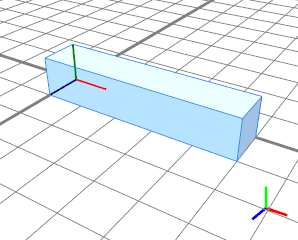

Absolute split

The absolute split cuts the geometry at absolute values.

The operation split(x) { 3 : Blue } splits the geometry along the x-dimension of the scope. The cube of length 5 is cut at an absolute value of 3 units and replaced with the successive cube shape Blue. 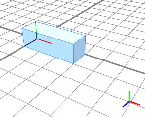Lot --> s(5, 1, 1) primitiveCube() split(x) { 3 : Blue(1) }
This example shows what happens if two absolute split values are used (3 units in green and 1 unit in blue). After the split the total resulting length is 3+1=4. 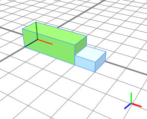Lot --> s(5, 1, 1) primitiveCube() split(x) { 3 : Blue(1) }
This example shows the effect of absolute values within a (limited) scope. The resulting shape Yellow has a length of 1 instead of 2 since there is a total length of 5. The rightmost shape Blue will not be generated. 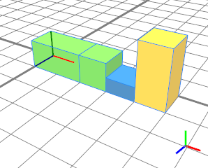split(x) { 2 : Green(1) | 1 : Green(1) | 1 : Blue(0.5) | 2 : Yellow(2) | 1 : Blue(1) }
No splits will be produced with negative or zero-sized values. Both Yellow shapes are not generated. Blue starts at 1.5. The last Green shape stops at the total length of 5. 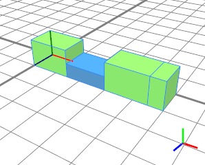split(x) { 1.5 : Green(1) | -2 : Yellow(1) | 1.5 : Blue(0.5) | 1.5 : Green(1) | 0 : Yellow(1) | 1.5 : Green(1) }

Relative split

The relative split uses scales relative to the scope size instead of absolute values. Relative values are denoted by the operator ' followed by a value between 0 and 1.

This example cuts the scope using the Golden Ratio. 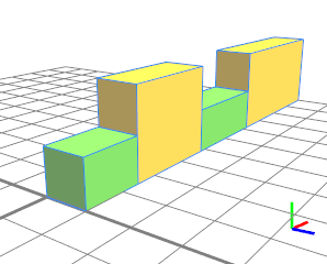split(x) { '0.382 : A | '0.618 : B } A --> split(x) { '0.382 : Green(1) | '0.618 : Yellow(2) } B --> split(x) { '0.382 : Green(1) | '0.618 : Yellow(2) }
This example shows a recursive split using the Golden Ratio. The recursion stops when the geometry gets too small for a further split. 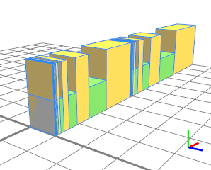split(x) { '0.382 : A | '0.618 : B } A --> split(x) { '0.382 : A | '0.618 : C } B --> split(x) { '0.382 : B | '0.618 : D } C --> split(x) { '0.382 : Green(1) | '0.618 : Yellow(2) } D --> split(x) { '0.382 : Green(1) | '0.618 : Yellow(2) }

Floating split

A floating split adapts values such that the entire space is filled. Floating splits are denoted by an operator ~.

In this example the split operation splits the cube of length 5 at 3 units (green). The remainder geometry is then cut at 1 unit. This time the floating operator ~ is used which expands the 1 unit over the remaining space of the first cut, i.e. 5-3=2 units (blue). 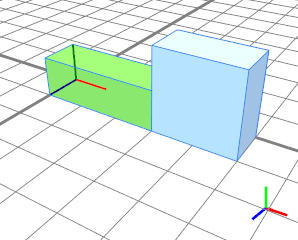split(x) { 3 : Green(1) | ~1 : Blue(2) }
The floating value 2 fills the space (3 units in yellow) between two absolute values (1 unit in blue). 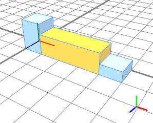split(x) { 1 : Blue(1.5) | ~2 : Yellow(1) | 1 : Blue(0.5) }
Multiple floating splits with same unit (each 1.5) are distributed evenly over the remaining scope space (2 units). 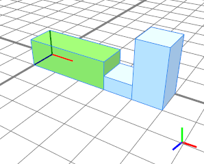split(x) { 3 : Green(1) | ~1.5 : Blue(0.5) | ~1.5 : Blue(2) }
Three floating splits are distributed evenly. 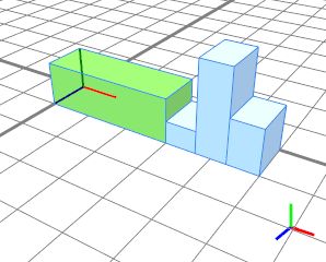split(x) { 3 : Green(1) | ~2 : Blue(0.5) | ~2 : Blue(2) | ~2 : Blue(1) }
If there is no space left for a floating split the corresponding shape is not generated (Blue in this case). 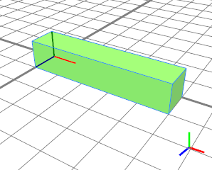split(x) { 5 : Green(1) | ~1 : Blue(1) }

Repeat split

The repeat split is used to repeat geometry within a given scope. It creates a rhythm: the repetitive use of a group of geometric objects in order to establish a recognizable pattern. A typical scenario is the alternating arrangement of windows and columns in the facades of common high rise office buildings. An asterisk * after the bracket denotes the repetitive split.

In the first example, a scope of length 10 is filled repetitively with a green shape with absolute length 2. Exactly 5 cubes of length 2 fit in the scope. Lot --> s(10, 1, 1) primitiveCube() split(x) { 2 : Green(1) }* A floating value of 2.1 generates the same result because a split to 5 successor shapes (with a length of 2 each) still approximates the target length of 2.1 best. 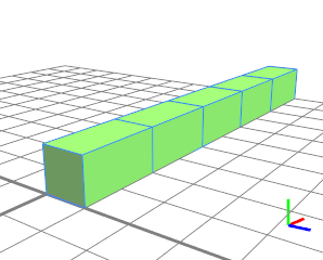split(x) { ~2.1 : Green(1) }*
A floating repeat split (green) is bordered by two absolute splits (blue). Note that the resulting length of the floating splits is (10-2)/3≈2.66 which is the best approximation for the target value 2.5. 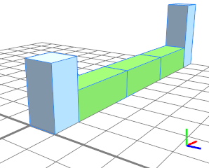split(x) { 1 : Blue(2) | { ~2.5 : Green(1) }* | 1 : Blue(3) }
The repetitive absolute split (green) will be evaluated first independently on which side of the split the repetition is denoted. The floating splits do not get any space to be generated. split(x) { { 2 : Green(1) }* | ~1 : Blue(2) } split(x) { ~1 : Blue(2) | { 2 : Green(1) }*
This example shows that a repeat split with absolute (or relative) values can be bordered by two neighboring floating (or absolute) splits. 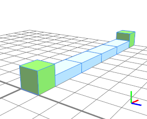split(x) { ~1 : Green(1) | { 2 : Blue(0.5) }* | ~1 : Green(1) }
The size of the first floating split and the size of the repetitive floating split is the same. The 2 units are equally distributed 4 times (blue) to the resulting length of (10-3)/4=1.75. 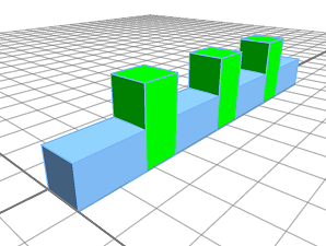split(x) { ~2 : Blue(1) | { 1 : Green(2) | ~2 : Blue(1) }* }

Repeat split - Patterns

Repeat operations can be used to create patterns. The following example shows that geometric objects can be grouped into a bracket and repeated.

A pattern is created and repeated. 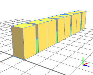split(x) { ~1 : Yellow(2) | 0.25 : Green(1) | ~1 : Yellow(2) }*
Repeating patterns can be inserted within other geometries. 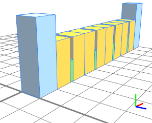split(x) { 1 : Blue(3) { ~1 : Yellow(2) | 0.2 : Green(1) | ~1 : Yellow(2) }* | 1 : Blue(3) }

Repeat split - Parallel

Repeat splits can be performed in parallel.

Two repeat splits (yellow and blue) bordered by floating splits (green). 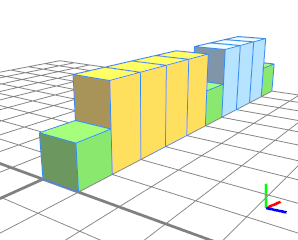split(x) { ~1 : Green(1) | { ~1 : Yellow(2) }* | ~1 : Green(1) | { ~1 : Blue(2) }* | ~1 : Green(1) }
Two successive repeat splits (green and yellow) bordered by absolute splits (blue). 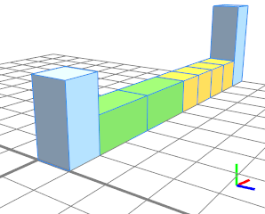split(x) { 1 : Blue(2) | { 2 : Green(1) }* | { 1 : Yellow(1) }* | 1 : Blue(3) }