Overview
The Stretch function enhances an image by changing properties such as brightness, contrast, and gamma through multiple stretch types.
The Stretch function uses the statistics from the rasters within the mosaic dataset; therefore, if you use this function, you must make sure statistics have been calculated.
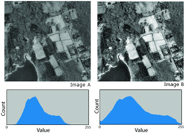
The following images show an example of a stretch. Histogram A represents the
pixel values in image A. By
stretching the values (shown in histogram B) across the entire
range, you can alter and visually enhance the appearance of the
image (image B).

Notes
The stretch type defines a histogram stretch that will be applied to the rasters to enhance their appearance. Stretching improves the appearance of the data by spreading the pixel values along a histogram from the minimum and maximum values defined by their bit depth. For example, an 8-bit raster dataset or mosaic dataset will be stretched from 0 to 255. Different stretches will produce different results in the raster display.
Parameters
Learn more about the stretch types
None
If the stretch type is None, no stretch method will be applied, even if statistics exist.
Standard deviation and percent clip
In many cases, you can assume that the majority of the pixel values fall within an upper and lower limit. Therefore, it's reasonable to trim off the extreme values. You can do this statistically by defining either a standard deviation or a clipping percent.
The standard deviation stretch type applies a linear stretch between the values defined by the standard deviation (n) value.
The percent clip stretch type applies a linear stretch between the defined percent clip minimum and percent clip maximum pixel values.
When you use either of these stretch types, all the values in the histogram falling outside the defined values are pushed to the ends. For example, assume your histogram has the same range of values as previously mentioned, 33 to 206, and you've defined a percent clip minimum and maximum of 2. If 2 percent at the low end are values 33 to 45, and 2 percent at the high end are values 198 to 206, the histogram will be redistributed to spread the values from 0 to 255. Values 33 to 45 become 0, values 198 to 206 become 255, and all others are spread in between. Similarly, if you define a 2 standard deviation, the values beyond the 2nd standard deviation become 0 or 255, and the remaining values are stretched between 0 and 255.
Minimum-maximum
This stretch type applies a linear stretch based on the output minimum and output maximum pixel values, which are used as the endpoints for the histogram. For example, in an 8-bit dataset, the minimum and maximum values could be 33 and 206. A linear stretch is used to distribute the values across 256 values, from 0 to 255. Features in the imagery are easier to distinguish as the pixel values are distributed across the entire histogram range, brightening and increasing the contrast of the image.
Sigmoidal
The Sigmoid contrast stretch is designed to highlight moderate pixel values in your imagery while maintaining sufficient contrast at the extremes. It places all of the pixel values along a sigmoidal function (an S-shaped curve). The result of this is less contrast in very bright and very dark areas, and more contrast in areas between these extremes. This is an ideal stretch for almost any image, and performs very well when there are clouds and water in the image.
The Strength Level determines how much of the sigmoidal function will be used in the stretch. A low value such as 1 will only use the middle portion of the curve, which tends to produce dull and faint colors. A high value such as 6 will use the entire curve, which tends to produce bold and sharp colors.
Learn more about gamma
Gamma refers to the degree of contrast between the midlevel gray values of a raster dataset. Gamma does not affect the black or white values in a raster dataset, only the middle values. By applying a gamma correction, you can control the overall brightness of a raster dataset. Additionally, gamma changes not only the brightness but also the ratios of red to green to blue.
Gamma values less than one decrease the contrast in the darker areas and increase the contrast in the lighter areas. This darkens the image without saturating the dark or light areas of the image. This helps bring out details in lighter features, such as building tops. Conversely, gamma values greater than one increase the contrast in darker areas, such as shadows from buildings. Gamma values greater than one can also help bring out details in lower elevation areas when working with elevation data.
In the following images, you can see the effect of adjusting the gamma
values used to display a raster dataset:
