Overview
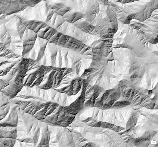
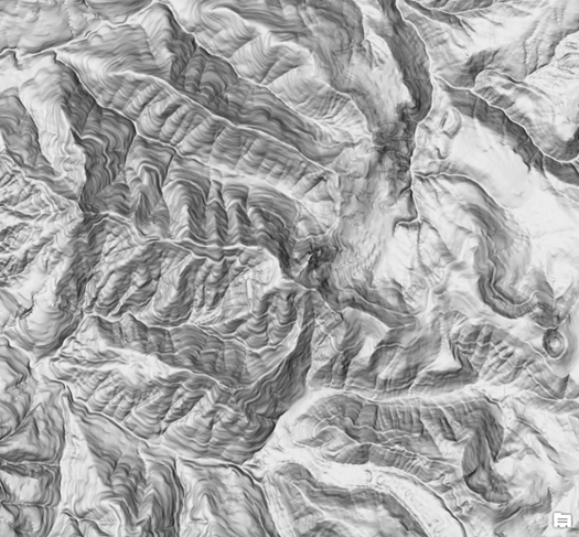
The hillshade function produces a grayscale 3D representation of the terrain surface, with the sun's relative position taken into account for shading the image. Hillshading is a technique for visualizing terrain determined by a light source and the slope and aspect of the elevation surface. It is a qualitative method for visualizing topography and does not give absolute elevation values. This function provides two options for generating hillshades: traditional and multidirectional. The traditional method calculates the hillshade using an illumination source from one direction using the altitude and azimuth properties to specify the sun's position. The multidirectional method combines light from multiple sources to represent the hillshaded terrain. The advantage of the multidirectional hillshade method is that more detail is displayed in areas typically affected by oversaturation and deep shadows than when using the traditional hillshade method.
By default, a grayscale color ramp is used to display a hillshaded elevation model. The following images display an elevation model using the traditional default hillshade method, followed by the multidirectional hillshade method.
Parameters
The Hillshade function has the following parameters:
| Parameter | Description |
|---|---|
| Raster | The input elevation dataset. |
| Hillshade Type | Controls the illumination source for the hillshade:
|
| Azimuth | Azimuth is the sun's relative position along the horizon (in degrees). This position is indicated by the angle of the sun measured clockwise from due north. An azimuth of 0 degrees indicates north, east is 90 degrees, south is 180 degrees, and west is 270 degrees. This parameter is only valid when Hillshade Type is Traditional. The default is 315 degrees, which is from the northwest. |
| Altitude | Altitude is the sun's angle of elevation above the horizon and ranges from 0 to 90 degrees. A value of 0 degrees indicates that the sun is on the horizon, that is, on the same horizontal plane as the frame of reference. A value of 90 degrees indicates that the sun is directly overhead. This parameter is only valid when Hillshade Type is Traditional. The default is 45 degrees above the horizon. |
| Scaling | The shaded result is scaled dynamically by adjusting the z-factor using one of two options:
|
| Z Factor | The z-factor is a scaling factor used to convert the elevation values for two purposes:
|
| Pixel Size Power | Pixel Size Power accounts for the altitude changes (or scale) as the viewer zooms in and out on the map display. It is the exponent applied to the pixel size term in the equation that controls the rate at which the Z Factor changes to avoid significant loss of relief. This parameter is only valid when the Scaling type is Adjusted. The default value is 0.664. |
| Pixel Size Factor | Pixel Size Factor accounts for changes in scale as the viewer zooms in and out on the map display. It controls the rate at which the Z Factor changes. This parameter is only valid when the Scaling type is Adjusted. The default value is 0.024. |
| Disable default edge pixel interpolation | Using this option avoids any resampling artifacts that may occur along the edges of a raster. The output pixels along the edge of a raster or beside NoData pixels will be populated with NoData; therefore, it is recommended that you use this parameter only with elevation mosaic datasets that have overlap. When overlapping pixels are available, the areas of NoData will display the overlapping pixel values instead of blank pixels.
The results from the function can be data dependent. If you observe tile boundary artifacts in your output, select the alternate condition of the check box. |
Learn more about how hillshade works
Hillshade type
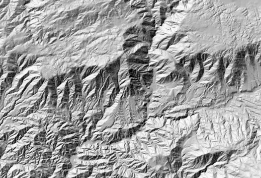
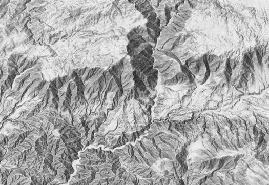
Multidirectional hillshade improves terrain visualization. It combines light from six different directions to represent an enhanced visualization of the terrain and to improve the appearance of regions with low relief. It improves the balance between the overexposed and shadow areas of the map. The output is suitable to use as a relief backdrop for topographical, soil, hydrological, land cover, or other thematic maps in which the data will be enhanced with topography.
The following images display the two types of hillshade:
- The top image shows the traditional hillshade result.
- The bottom image shows the multidirectional hillshade result.
For more information about multidirectional hillshade, see Multi-Directional Hillshade Makes Your Maps Pop.
Azimuth and altitude
The properties altitude and azimuth together indicate the sun's relative position that will be used for creating any 3D model (hillshade or shaded relief). Altitude is the sun's angle of elevation above the horizon and ranges from 0 to 90 degrees. A value of 0 degrees indicates that the sun is on the horizon, that is, on the same horizontal plane as the frame of reference. A value of 90 degrees indicates that the sun is directly overhead.
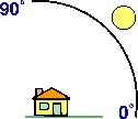
Azimuth is the sun's relative position along the horizon (in degrees). This position is indicated by the angle of the sun measured clockwise from due north. An azimuth of 0 degrees indicates north, east is 90 degrees, south is 180 degrees, and west is 270 degrees.
Scaling and pixel size
The shaded result is scaled dynamically by adjusting the z-factor using one of two options:
- None—No scaling is applied. This is ideal for a single raster datasets covering a local area. This is not recommended for worldwide datasets or multi-scale maps as it will produce a fairly flat relief at small scales.
- Adjusted—This applies a nonlinear adjustment using the default Pixel Size Power and Pixel Size Factor values, which accounts for the altitude changes (scale) as the viewer zooms in and out. These values are recommended when using the worldwide dataset.
The z-factor is adjusted using the following equation:
Adjusted Z-Factor = (Z Factor) + (Pixel Size)(Pixel Size Power) × (Pixel Size Factor)
Slope is a factor of pixel size. With larger pixels, the slope value gets smaller since the slope represents the average slope over a larger distance. As a result, at small scales, features appear flat. Cartographically this results in significant loss of relief. To compensate for this, the Z Factor parameter can be changed according to scale. The relationship is exponential rather than linear. Changing Pixel Size Power and Pixel Size Factor changes the rates at which Z Factor changes. This means that the z-factor needs to be set appropriate to the scale.
Z-factor
The z-factor is a scaling factor used to convert the elevation values for two purposes:
- To convert the elevation units (such as meters or feet) to the horizontal coordinate units of the dataset, which may be feet, meters, or degrees
- To add vertical exaggeration for visual effect
Unit conversion
If the units for the z (elevation) units are the same as the x,y (linear) units, then the z conversion factor is 1. If your dataset is using a projected coordinate system, your scaling is set to None, and your elevation and linear units are different, then you will need to define a z conversion factor to account for the difference.
To convert from feet to meters or vice versa, see the table below. For example, if your DEM's elevation units are feet and your mosaic dataset's units are meters, you would use a value of 0.3048 to convert your elevation units from feet to meters (1 foot = 0.3048 meters).
Scaling and pixel size
| Conversion type | Conversion factor |
|---|---|
From feet to meters | 0.3048 |
From meters to feet | 3.28084 |
If your data is using a geographic coordinate system (such as a DTED in GCS_WGS 84), where the linear units are in degrees and your elevation is in meters, use a conversion factor of 1, and the system will automatically convert your linear degrees to meters. If your elevation units are not in meters, use the Unit Conversion function to convert your elevation to meters before using this function.
Note:
When your scaling is set to Adjusted, you can use the Z Factor to convert z units to meters, and ArcGIS will automatically adjust the latitude and longitude to meters.
Vertical exaggeration
To apply vertical exaggeration, you must multiply the conversion factor by the exaggeration factor. For example, if both elevation and dataset coordinates are meters and you want to exaggerate by a multiple of 10, the scaling factor would be the unit conversion factor (1.0) multiplied by the vertical exaggeration factor (10.0), which would be a z-factor of 10. If the elevation units are meters and the dataset is geographic (degrees), you would multiply the unit conversion factor (1.0) by the exaggeration factor (10.0), which would be a z-factor of 10. If your elevation units are not in meters, use the Arithmetic function to convert your elevation to meters before using this function. Then multiply the unit conversion factor (1.0) by the exaggeration factor (10.0), which would be a z-factor of 10.
Remove edge effect
Using this option will avoid any resampling artifacts that may occur along the edges of a raster. The output pixels along the edge of a raster or beside pixels without a value will be populated with NoData; therefore, it is recommended that this option be used only when there are other rasters with overlapping pixels available. When overlapping pixels are available, these areas of NoData will display the overlapping pixel values instead of being blank.
- Unchecked—Bilinear resampling will be applied uniformly to resample your hillshade. This is the default.
- Checked—Bilinear resampling will be used within the hillshade except along the edges of the rasters or beside pixels of NoData. These pixels will be populated with NoData and display the elevation values of the overlapping dataset, thus reducing any sharp edge effects that may occur.