The steps in this lesson outline how to create a big data analytic using ArcGIS Velocity. The example uses the role of a transportation planner looking to better understand motor vehicle accidents involving bicyclists over a multiyear period. The findings are used to help identify where the construction of new bicycle-friendly infrastructure such as bike lanes or lane barriers would generate the greatest impact for cyclist safety.
As you work through the steps, you will create a big data analytic, configure its data source, configure tools, and generate an output feature layer containing analytic results that can be viewed in a web map.
This lesson is designed for beginners. You must connect to an ArcGIS Online organization with access to Velocity. The estimated time to complete this lesson is 30 minutes.
Create a big data analytic
To begin, do the following:
- In a web browser, open ArcGIS Velocity and sign in to an ArcGIS Online organization that is licensed for Velocity.
Google Chrome or Mozilla Firefox is recommended.
Note:
If you encounter issues signing in, contact your ArcGIS organization administrator. You may need to be assigned a role with privileges to use ArcGIS Velocity.
The Home page appears.
- From the main menu, under Analytics, click Big Data to access the Big Data Analytics page.
Tip:
The Getting Started section on the Home page has a Create big data analytic shortcut button under Big Data Analytic.
On the Big Data Analytics page, you can perform the following actions on existing big data analytics:
- Review
- Create
- Start
- Stop
- Check status
- Edit
- Clone
- Delete
- Share
- View logs
- Check metrics
- Click Create big data analytic.
The configuration wizard opens and data source type options appear.
You have signed in to Velocity and started the process to create a big data analytic in a configuration wizard. The next step is to configure its data source.
Configure the data source
The data used in this lesson can be downloaded from the New York City (NYC) OpenData site. The complete dataset of more than 1.5 million records was downloaded from this site in comma-separated values (CSV) format. For this lesson, the .csv file is hosted on a public Amazon S3 bucket. Connection information is provided in the steps below.
A big data analytic requires a data source. Complete the following steps to configure a data source:
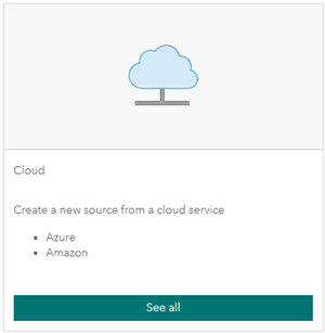
- For Select a type of data source, click See all in the Cloud category.
Note:
All big data analytics must have at least one input data source.
- Under Cloud options, choose Amazon S3.
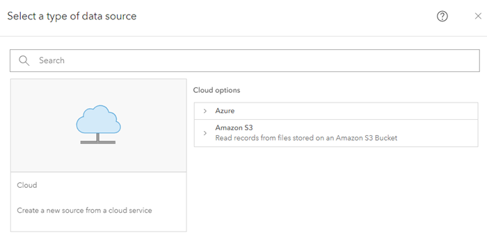
Learn more about Azure Blob Store, Azure Cosmos DB, or Amazon S3.
- On the Configure Amazon S3 dialog box, for Configure Amazon S3 Bucket, set the parameters as follows:
- For Access mode, choose Public.
- For Bucket name, type arcgis-velocity-public.
- For Region, choose US West (Oregon).
- For Folder path (optional), type /nyc-motor-vehicle-collisions.
- For Dataset, type NYPD_Motor_Vehicle_Collisions.csv.
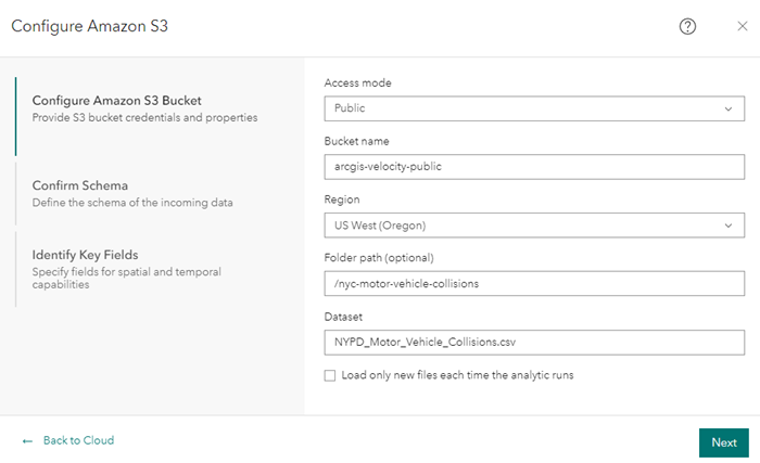
- Click Next to apply the Amazon S3 bucket parameters.
The data source validates and returns sampled event data for review. The next step is to confirm the data schema.
Amazon S3 is configured as the data source.
Confirm the data schema
With the Amazon S3 bucket parameters set, you can confirm the data schema. When configuring a data source, it is important to define the schema of the data being loaded. Velocity defines the schema when it samples the source data, including the values for the Data format, Field delimiter, Field Type, and Field Name options.
- For Confirm Schema, review and ensure that the schema of the data is similar to the following illustration:
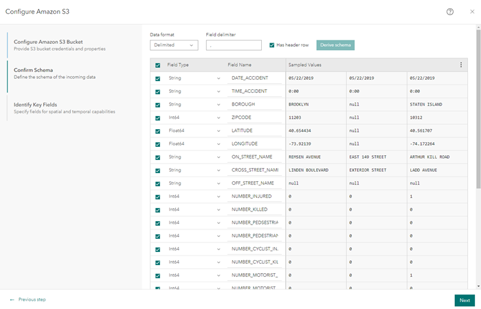
Velocity tested the connection to the data source, sampled the first few data records, and interpreted the schema of the data based on the sampled records. You can change the Data format, Field delimiter, Field Type, and Field Name values if necessary to ensure a valid schema. For the purposes of this lesson, accept the default schema parameters.
- Click Next to ensure the schema as sampled.
Identify key fields
In this step, fields are specified for spatial and temporal capabilities by choosing values for the Location, Date and Time, and Tracking parameters so that Velocity can properly construct geometry, date information, and a unique identifier for the data.
Complete the following steps to identify the key fields:
- For Location type, choose X/Y fields.
- For X (longitude), choose Longitude.
- For Y (latitude), choose Latitude.
- For Z (altitude), choose None.
- For Spatial reference, leave the default GCS WGS 1984 value.
- For Does your data have date fields?, choose No.
This parameter can be used to set a start and end date or date-time field in the data source. If the incoming data includes date information in a string format, a date format is required. For this lesson's purposes, no date or time information is specified.
- For Track ID, choose Data does not have a Track ID.
This parameter can be used to designate a track ID field in the data source. For this lesson, don't define a track ID.

- Click Complete to create the data source.
The Amazon S3 data source is added to the analytic editor.
Create the big data analytic
With the data source added to the analytic editor, you can create the big data analytic.
- On the New Big Data Analytic page, click Create analytic.
The Create Analytic dialog box appears.
- For Title, type NYC Cyclist Accidents.
- For Summary, type Process motor vehicle accidents to identify and analyze those involving cyclists.
- For Folder, choose the folder where you want to create the big data analytic.
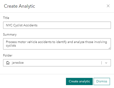
- Click Create analytic to create the analytic.
The analytic editor reappears with more options on the toolbar.
Add and configure an analytic tool
With the new analytic created, you can add tools to perform the big data analysis on the New York City cyclist accident data. Velocity allows you to configure an analytic pipeline.
First, add the Calculate Field tool and then a TotalCyclistCasualties field that sums the values in the NUMBER_CYCLIST_INJURED and NUMBER_CYCLIST_KILLED fields for each individual record from the data source.
Complete the following steps to configure sequential tools to better understand motor vehicle accidents involving injuries to cyclists:
- From the Add Node menu, click Manage Data and choose the Calculate Field tool.
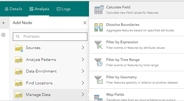
The Calculate Field tool is added to the analytic editor.
- Connect the Amazon S3 data source to the Calculate Field tool.

If necessary, reposition the tool and data source in the analytic editor to facilitate a connection. A connection ensures that the Calculate Field tool knows what data source to use.
- Double-click the Calculate Field tool to access its properties.
- Click Add field calculation and choose New field.
- For Field, type TotalCyclistCasualties.
- Click the Type drop-down arrow and choose Int64.
This specifies the field type is a 64-bit integer field.
- Click Configure an Arcade expression to open the Configure an Arcade expression dialog box.
- Use the Arcade expression builder and type $feature.NUMBER_CYCLIST_INJURED+$feature.NUMBER_CYCLIST_KILLED.
- Click Run to run the Arcade expression.
The result should resemble the following illustration:
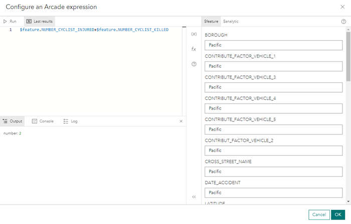
- Click OK to save the expression.
- Click Dismiss field calculation to return to the Calculate field properties page
- Click Add field calculation to add the new field calculation to the Calculate Field tool.
Tip:
You can add more field calculations as necessary. This lesson only uses the one.
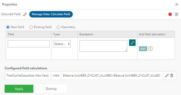
- Click Apply to apply the calculation to the Calculate Field tool properties.
The Calculate Field tool is configured and connected to the Amazon S3 data source. Next, you can filter the New York City motor vehicle accident data to identify the accidents with valid location coordinates that resulted in a cyclist injury or death.
- In the analytic editor, click Save to save the big data analytic configuration.
- From the Add Node menu, click Manage Data and choose the Filter by Expression tool.
A Filter by Expression tool is added to the analytic editor.
- Drag the Filter by Expression tool after the Calculate Field tool and connect the two nodes.

- Double-click the Filter by Expression tool to open the properties and configure as follows:
- Click Configure an Arcade expression to open the Configure an Arcade expression dialog box.
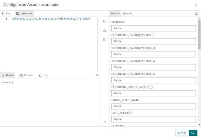
- Use the Arcade expression builder or type $feature.TotalCyclistCasualties>0 && $feature.LATITUDE>0.
Records with invalid coordinates exist in this dataset. These records can be ignored by filtering out records in which the latitude value is less than or equal to 0.
- Click Run to run the Arcade expression.
The result should resemble the following illustration:
- Click OK to return to the Filter by Expression tool properties.
- Click Apply to apply the expression.
The filter is added. Next, you add the Aggregate Points tool, which aggregates points spatially to represent the number of accidents involving cyclist injury or death as regular hexagonal bins.
- From the Add Node menu, click Summarize Data and choose the Aggregate Points tool.
The Aggregate Points tool is added to the analytic editor.
- In the analytic editor, click Save to save the updated big data analytic configuration.
- Drag the Aggregate Points tool after the Filter by Expression tool and connect the two nodes.

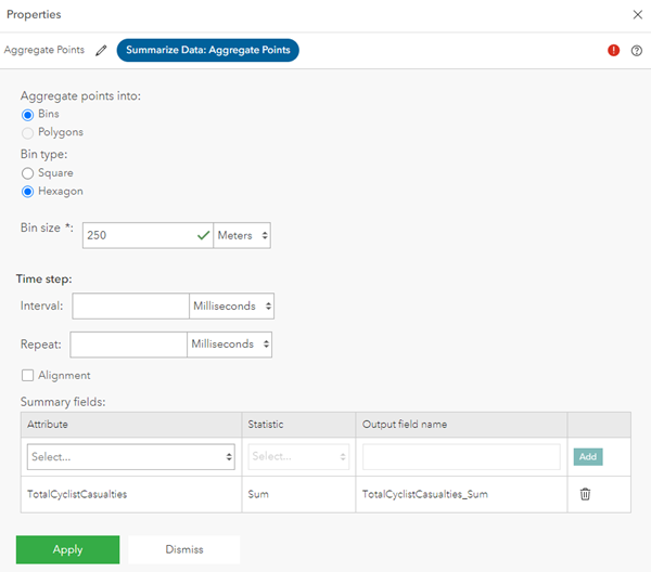
- Double-click the Aggregate Points tool to open its properties and configure as follows:
- For Aggregate points into, choose Bins.
- For Bin type, choose Hexagon.
- For Bin size, type 250 and keep the unit of measurement set to Meters.
- Leave the Time step section as is and in the Summary fields section, click Add summary field.
The properties pane appears.
- For Attribute, choose TotalCyclistCasualties.
- For Statistic, choose Sum.
- For Output field name, leave the default TotalCyclistCasualties_Sum.
- Click Add summary field to add the summary field.
- Click Apply to apply the tool properties.
You have successfully added three analytic tools that process the accident data. Next, you add an output.
Configure a feature layer output
With the data source and analytic tools created, the last step in this lesson is to add an output that sends the processed event data to a feature layer, which can be visualized in a web map.
Note:
The spatiotemporal feature layer name must be unique within an organization.
In Velocity, the spatiotemporal feature layer name must be different from the feed and stream layer names. If there is a duplicate name, you cannot create a real-time or big data analytic in Velocity. This only applies to Velocity feature layer outputs; it does not apply to ArcGIS Online hosted feature layers.
To add an output, complete the following steps:
- From the Add Node menu, click Outputs and choose Feature Layer (new).
The Configure Feature Layer (new) dialog box appears.
- For Configure Feature Layer, configure the properties as follows:
- Turn on the Store data in spatiotemporal feature layer toggle button.
- For Data storage method, choose Add all new features.
If you were working with a data source that had a track ID defined, you'd use the Keep only latest feature for each Track ID value method. With this storage method, each time a new feature is received for a certain track ID, the stored feature associated with that track ID is replaced by the new feature.
- For Each time the analytic runs, choose Replace existing features and schema.
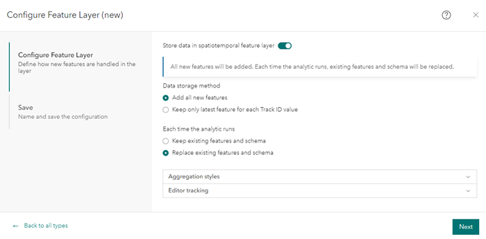
Each time a big data analytic runs, the features and schema in the output feature layer are overwritten. This is useful for developing and testing big data analytics and adding, removing, or changing tools between analytic runs.
Note:
Choose the Keep existing features and schema option to append records to the feature layer output each time the big data analytic runs.
- Click Next.
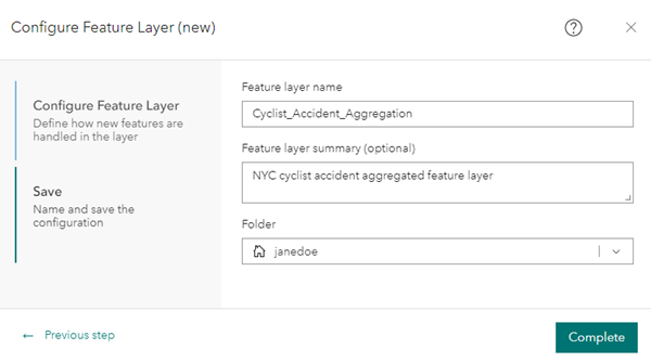
- For Save, for Feature layer name, type Cyclist_Accident_Aggregation.
- For Feature layer summary (optional), type NYC cyclist accident aggregated feature layer.
- For Folder, choose the folder where you want to save the feature layer.
- Click Complete to save the new output.
The new Cyclist_Accident_Aggregation output is added to the analytic editor.
- Drag the Cyclist_Accident_Aggregation output after the Aggregate Points tool and connect the two nodes.
Tip:
You can move the nodes to make the model more visually appealing.

- Click Save to save the NYC Cyclist Accidents big data analytic.
You have successfully added a new feature layer output, Cyclist_Accident_Aggregation, to view the accident data in a web map.
Start the big data analytic
Now that you have successfully configured a big data analytic with the necessary nodes, you can start the analytic. The analytic loads more than 1.5 million records from the .csv file using a defined schema, processes the event data through a variety of tools, and writes the analysis output to a new feature layer.
Complete the following steps to run the analytic once:
- In the analytic editor, click Start to start the NYC Cyclist Accidents big data analytic.

The Start button becomes a Stop Initialization button and then a Stop button, indicating that the analytic has started and is running.
Note:
Feeds and real-time analytics in Velocity remain running once they are started. Big data analytics, on the other hand, run until the analysis is complete and stop automatically. Big data analytics can be configured to run in a recurring manner using the options available from the Schedule drop-down menu in the analytic editor. Options include the ability to run the analytic once, periodically, or at a recurring time.
- Monitor the analytic until the Stop button reverts to Start.
This indicates that the analytic ran once, is now finished, and is no longer running. Additionally, you can monitor the status of big data analytics from the Big Data Analytics page.
You have successfully initialized the NYC Cyclist Accidents big data analytic.
Explore the analytic results in a web map
When you started the big data analytic in the previous section, an output feature layer was created. Open that output feature layer in a web map and review the results of the big data analysis on the NYC cyclist accident data.
- From the main menu, under Output, click the Layers tab to open the Layers page.
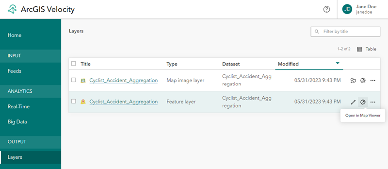
- Browse to the Cyclist_Accident_Aggregation feature layer in the list and click Open in Map Viewer to review the feature layer in a web map.
Note:
Output layers created by real-time and big data analytics do not appear on the Layers page until the analytic runs and has generated an output.
- Zoom in to focus on the data for New York City, USA.
- On the Content (dark) toolbar, click Basemap and change the basemap to Dark Gray Canvas.
- For the Cyclist_Accident_Aggregation feature layer, click Styles.
- For Choose attributes, choose Count from the drop-down menu, and click Add.
- For Pick a style, choose Counts and Amounts (color) if necessary, and click Style options.
- In Style options, click Symbols style.
- For Colors, change the color ramp to Reds and yellows, click Done, and close the symbol style.
- Scroll to the end of the Style options and click the Classify Data toggle to group the data and highlight areas with higher cyclist-related injuries.
- Under the Classify Data toggle button, click the Method drop-down arrow and choose Standard Deviation, and set the class size to 1 standard deviation.
- Accept the other default properties and then click Done.

The web map is set and can be reviewed. You can pan and zoom around the web map to explore the results of the big data analysis and identify areas that had more cyclist-related injuries and deaths and the areas with fewer.
Additional resources
In this lesson, you created and ran a big data analytic that analyzed roughly 1.5 million cyclist accidents to identify areas in New York City with the highest number of accidents. With these results, you can make better informed decisions on where new bicycle infrastructure would have the greatest impact.
Additional resources are available as you continue to work with Velocity including the following: