Available with Spatial Analyst license.

Available with 3D Analyst license.

The tool calculates the second derivative value of the input surface on a cell-by-cell basis.

Note:

The Curvature tool fits a plane to the nine local cells, but a plane may not be a good descriptor of the landscape and may mask or exaggerate natural variations of interest. The tool fits a surface to the neighborhood of cells instead of a plane, which provides a more natural fit to the terrain.

The Curvature tool uses a 3 by 3 window of cells to compute the value, while the Surface Parameters tool allows window sizes from 3 by 3 to 15 by 15 cells. Larger window sizes are useful with high resolution elevation data to capture land surface processes at an appropriate scale. Surface Parameters also provides an adaptive window option that evaluates the local variability of the terrain and identifies the largest appropriate neighborhood size for each cell. This can be useful with gradual homogeneous terrain interrupted by streams, roads, or sharp breaks in slope.

The Surface Parameters tool includes three curvature types, which use updated formulas and create different results from the Curvature tool.

For each cell, a fourth-order polynomial of the form:

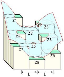
 Z = Ax²y² + Bx²y + Cxy² + Dx² + Ey² + Fxy + Gx + Hy + I

is fit to a surface composed of a 3 x 3 window. The coefficients a, b, c, and so on, are calculated from this surface.

The relationships between the coefficients and the nine values of elevation for every cell numbered as shown on the diagram are as follows:

Curvature values diagram

A = [(Z1 + Z3 + Z7 + Z9) / 4  - (Z2 + Z4 + Z6 + Z8) / 2 + Z5] / L4 
B = [(Z1 + Z3 - Z7 - Z9) /4 - (Z2 - Z8) /2] / L3 
C = [(-Z1 + Z3 - Z7 + Z9) /4 + (Z4 - Z6)] /2] / L3 
D = [(Z4 + Z6) /2 - Z5] / L2 
E = [(Z2 + Z8) /2 - Z5] / L2 
F = (-Z1 + Z3 + Z7 - Z9) / 4L2 
G = (-Z4 + Z6) / 2L 
H = (Z2 - Z8) / 2L 
I = Z5

The output of the is the sum of the second derivatives of the surface.

Standard Curvature = -100 * ([d2z/dx2] + [d2z/dy2])

Curvature is sometimes described ambiguously as the second derivative of the surface, or “slope of the slope”. This terminology refers to the profile curvature.

Profile Curvature = -2(D + E) * 100

From an applied viewpoint, the output of the tool can be used to describe the physical characteristics of a drainage basin in an effort to understand erosion and runoff processes. The slope affects the overall rate of movement downslope. Aspect defines the direction of flow. The profile curvature affects the acceleration and deceleration of flow and, therefore, influences erosion and deposition. The planform curvature influences convergence and divergence of flow.

Interpreting results from Curvature

Displaying contours over a raster may help with understanding and interpreting the data resulting from the execution of the tool. An example of the process follows, with the tools identified and the settings used.

1. Create a curvature raster from the surface raster with the Curvature tool:

   Input raster : elev_ras

   Output curvature raster : curv_ras

   Z factor : 1

   Output profile curve raster : profile_ras

   Output plan curve raster : plan_ras

2. Create contours of the surface raster with the Contour tool:

   Input raster : elev_ras

   Output polyline features : cont_lines

   Contour interval : 100

   Base contour : ""

   Z factor : 1

3. Create a slope raster from the surface raster with the Slope tool:

   Input raster : elev_ras

   Output raster : slope_ras

   Output measurement : DEGREE

   Z factor : 1

4. Then create contours of the slope raster with the Contour tool:

   Input raster : slope_ras

   Output polyline features : cont_slope

   Contour interval : 5

   Base contour : ""

   Z factor : 1

5. Add the curvature raster as a layer to the map display. Overlay the two contour feature datasets just created and apply different color symbology for each.

Should I use the Surface Parameters tool?

If the Input raster parameter value (in_raster in Python) is high resolution with a cell size of less than a few meters, or particularly noisy, consider using the Surface Parameters tool and its user-defined neighborhood distance option instead of the immediate 3 by 3 neighborhood of this tool. Using a larger neighborhood can minimize the effect of noisy surfaces. Using a larger neighborhood can also better represent landforms and surface characteristics when using high resolution surfaces.

References

Moore, I. D., R. B. Grayson, and A. R. Landson. 1991. Digital Terrain Modelling: A Review of Hydrological, Geomorphological, and Biological Applications. Hydrological Processes 5: 3–30.

Zeverbergen, L. W., and C. R. Thorne. 1987. Quantitative Analysis of Land Surface Topography. Earth Surface Processes and Landforms 12: 47–56.