Available with Spatial Analyst license.
Available with 3D Analyst license.
The tool identifies the steepness at each cell of a raster surface. The lower the slope value, the flatter the terrain; the higher the slope value, the steeper the terrain.
Note:
The Surface Parameters tool provides a newer implementation of slope and is recommended to be used instead of the Slope tool. The Slope tool fits a plane to the nine local cells, but a plane may not be a good descriptor of the landscape and may mask or exaggerate natural variations of interest. The Surface Parameters tool fits a surface to the neighborhood of cells instead of a plane, which provides a more natural fit to the terrain.
The Slope tool uses a 3 by 3 window of cells to compute the value, while the Surface Parameters tool allows window sizes from 3 by 3 to 15 by 15 cells. Larger window sizes are useful with high resolution elevation data to capture land surface processes at an appropriate scale. Surface Parameters also provides an adaptive window option that evaluates the local variability of the terrain and identifies the largest appropriate neighborhood size for each cell. This can be useful with gradual homogeneous terrain interrupted by streams, roads, or sharp breaks in slope.
You can continue to use the traditional approach of the Slope tool if you need the results to exactly match previous tool runs or if fast execution time is more important than a better algorithm.
The output slope raster can be calculated in two types of units, degrees or percent (percent rise). The percent rise can be better understood if you consider it as the rise divided by the run, multiplied by 100. Consider triangle B below. When the angle is 45 degrees, the rise is equal to the run, and the percent rise is 100 percent. As the slope angle approaches vertical (90 degrees), as in triangle C, the percent rise begins to approach infinity.

The Slope tool is most frequently run on an elevation dataset as the following images show. Steeper slopes are shaded darker brown on the output slope raster.
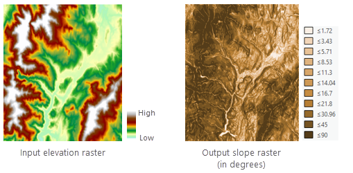
The tool can also be used with other types of continuous data, such as population, to identify sharp changes in value.
Calculation methods and the edge effect
Two methods are available for slope computation. You can choose between performing Planar or Geodesic calculations with the Method parameter.
For the planar method, the slope is measured as the maximum rate of change in value from a cell to its immediate neighbors. The calculation is performed on a projected flat plane using a 2D Cartesian coordinate system. The slope value is calculated using a third-order finite difference estimator.
With the geodesic method, the calculation will be performed in a 3D Cartesian coordinate system by considering the shape of earth as an ellipsoid. The slope value is calculated by measuring the angle between topographic surface and the referenced datum.
Both planar and geodesic computations are performed using a 3 by 3 cell neighborhood (moving window). For each neighborhood, if the processing (center) cell is NoData, the output is NoData. The computation also requires at least seven cells neighboring the processing cell have valid values. If there are fewer than seven valid cells, the calculation will not be performed, and the output at that processing cell will be NoData.
The cells in the outermost rows and columns of the output raster will be NoData. This is because along the boundary of the input dataset, those cells do not have enough valid neighbors.
Planar method
The slope is computed as the rate of change (delta) of the surface in the horizontal (dz/dx) and vertical (dz/dy) directions from the center cell to each adjacent cell. The basic algorithm used to calculate the slope is as follows:
slope_radians = ATAN ( √ ([dz/dx]2 + [dz/dy]2) )Slope is commonly measured in units of degrees, which uses the following algorithm:
slope_degrees = ATAN ( √ ([dz/dx]2 + [dz/dy]2) ) * 57.29578Note:
The value 57.29578 shown here is a truncated version of the result from 180/pi.
The slope algorithm can also be interpreted as follows:
slope_degrees = ATAN (rise_run) * 57.29578- where:
rise_run = √ ([dz/dx]2 + [dz/dy]2]
The values of the center cell and its eight neighbors determine the horizontal and vertical deltas. The neighbors are identified as letters from a to i, with e representing the cell for which the slope is being calculated.
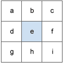
The rate of change in the x direction for cell e is calculated with the following algorithm:
[dz/dx] = ((c + 2f + i)*4/wght1 - (a + 2d + g)*4/wght2) / (8 * x_cellsize)- where:
wght1 and wght2 are the horizontal weighted counts of valid cells.
For instance, if:
- c, f, and i all have valid values, wght1 = (1+2*1+1) = 4.
- i is NoData, wght1 = (1+2*1+0) = 3.
- f is NoData, wght1 = (1+2*0+1) = 2.
Similar logic applies to wght2, except the neighbor locations are a, d, and g.
The rate of change in the y direction for cell e is calculated with the following algorithm:
[dz/dy] = ((g + 2h + i)*4/wght3 - (a + 2b + c)*4/wght4) / (8 * y_cellsize)- where:
wght3 and wght4 are the same concept as in the [dz/dx] computation.
Planar slope calculation example
As an example, the slope value of the center cell of the moving window shown below will be calculated.
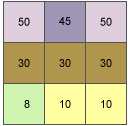
The rate of change in the x direction for the center cell e is:
  [dz/dx] = ((c + 2f + i)*4/wght1 - (a + 2d + g)*4/wght2) / (8 * x_cellsize)
          = ((50 + 60 + 10)*4/(1+2+1) - (50 + 60 + 8)*4/(1+2+1)) / (8 * 5)
          = (120 - 118) / 40
          = 0.05
The rate of change in the y direction for cell e is:
  [dz/dy] = ((g + 2h + i)*4/wght3 - (a + 2b + c)*4/wght4) / (8 * y_cellsize)
          = ((8 + 20 + 10)*4/(1+2+1) - (50 + 90 + 50)*4/(1+2+1)) / (8 * 5)
          = (38 - 190 ) / 40
          = -3.8
Taking the rate of change in the x and y direction, the slope for the center cell e is calculated using the following:
  rise_run = √ ([dz/dx]2 + [dz/dy]2)
           = √ ((0.05)2 + (-3.8)2)
           = √ (0.0025 + 14.44)
           = 3.80032
slope_degrees = ATAN (rise_run) * 57.29578
= ATAN (3.80032) * 57.29578
= 1.31349 * 57.29578
= 75.25762The integer slope value for cell e is 75 degrees.
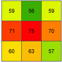
Geodesic method
The geodesic method measures slope in a geocentric 3D coordinate system—also called the Earth Centered, Earth Fixed (ECEF) coordinate system—by considering the shape of the earth as an ellipsoid. The computation result will not be affected by how the dataset is projected. It will use the z-units of the input raster if they are defined in the spatial reference. If the spatial reference of the input does not define the z-units, you will need to do so with the z-unit parameter. The geodesic method produces a more accurate slope than the planar method.
Geodesic coordinate transformation
The ECEF coordinate system is a 3D right-handed Cartesian coordinate system with the center of the earth as the origin, where any location is represented by X, Y and Z coordinates. See the following figure for an example of a target location T expressed with geocentric coordinates.
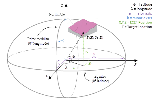
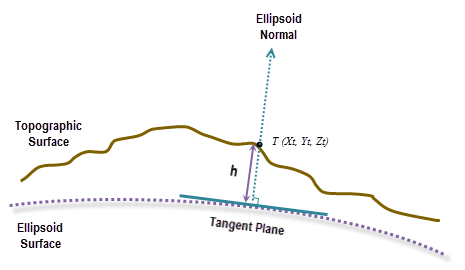
The geodesic computation uses an X, Y, Z coordinate that is calculated based on its geodetic coordinates (latitude φ, longitude λ, height h). If the coordinate system of the input surface raster is a projected coordinate system (PCS), the raster is first re-projected to a geographical coordinate system (GCS) where each location has a geodetic coordinate, and then transformed to the ECEF coordinate system. The height h (z-value) is the ellipsoid height referenced to the ellipsoid surface. See the illustration graphic below.
To transform to ECEF coordinates from a geodetic coordinate (latitude φ, longitude λ, height h), use the following formulas:
X = (N(φ)+h)cosφcosλY = (N(φ)+h)cosφsinλZ = (b2/a2*N(φ)+h)sinφ- where:
- N( φ ) = a2/ √(a2cosφ2+b2sinφ2)
- φ = latitude
- λ = longitude
- h = ellipsoid height
- a = major axis of the ellipsoid
- b = minor axis of the ellipsoid
The ellipsoid height h is in meters in the above formulas. If your input raster's z-unit is specified in any other unit, it will be internally transformed to meter.
Slope computation
The geodesic slope is the angle formed between the topographic surface and the ellipsoid surface. Any surface parallel to the ellipsoid surface has a slope of 0. To calculate the slope at each location, a 3 by 3 cell neighborhood plane is fitted around each processing cell using the Least Squares Method (LSM). The best fit in the LSM minimizes the sum of squared difference (dzi) between the actual z-value and the fitted z-value. See the illustration below for an example.
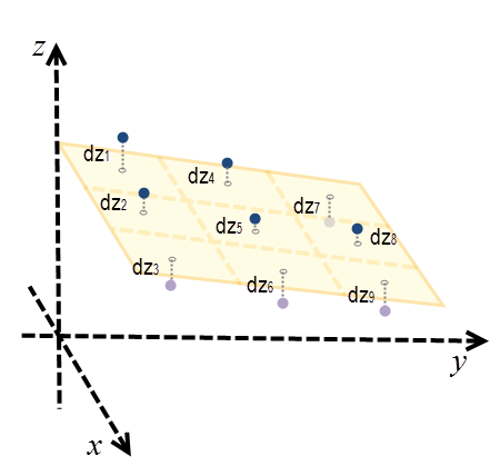
Here, the plane is represented as z = Ax + By + C. For each cell center, dzi is the difference between the actual z-value and the fitted z-value.
The plane is best fitted when ∑9i=1dzi2 is minimized.
After the plane is fitted, a surface normal is calculated at the cell location. At the same location, an ellipsoid normal perpendicular to the tangent plane of the ellipsoid surface is also calculated.
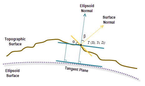
The slope, in degrees, is calculated from the angle between the ellipsoid normal and the topographic surface normal, represented as β here. From the illustration above, the angle α is the geodesic slope, which is the same as angle β, pursuant to the law of congruent geometry.
To calculate slope in percent rise, the following formula is used:
Slope_PercentRise = ATAN(β) * 100%Should I use the Surface Parameters tool?
If the Input raster parameter value (in_raster in Python) is high resolution with a cell size of less than a few meters, or particularly noisy, consider using the Surface Parameters tool and its user-defined neighborhood distance option instead of the immediate 3 by 3 neighborhood of this tool. Using a larger neighborhood can minimize the effect of noisy surfaces. Using a larger neighborhood can also better represent landforms and surface characteristics when using high resolution surfaces.
Use of a GPU
For the Geodesic method, this tool is capable of delivering increased performance if you have certain GPU hardware installed on your system. See the GPU Processing with Spatial Analyst section for details on how this is supported, how to configure it, and how to enable it.
References
Marcin Ligas, and Piotr Banasik, 2011. Conversion between Cartesian and geodetic coordinates on a rotational ellipsoid by solving a system of nonlinear equations (GEODESY AND CARTOGRAPHY), Vol. 60, No 2, 2011, pp. 145-159
B. Hofmann-Wellenhof, H. Lichtenegger and J. Collins, 2001. GPS - theory and practice. Section 10.2.1. p. 282.
David Eberly 1999. Least Squares Fitting of Data (Geometric Tools, LLC), pp. 3.