In the Rescale by Function tool, the transformation function is applied to the input values between (and including) the specified lower and upper threshold values. How the lower and upper thresholds are set relative to the input raster values can produce very different results. There are three general use cases when specifying the lower and upper thresholds to the input values:
- The lower and upper threshold equal the lowest and highest input values (data dependent).
General use case: Determine the relative suitability of the cells for deer within a dataset.
- The lower threshold is greater than the lowest input value or the upper threshold is less than the highest input value (the thresholds are contained within the data).
General use case: Determine the relative suitability of the cells for deer within a dataset that contains values where the deer cannot live.
- The lower threshold is lower than the lowest input value or the upper threshold is greater than the highest input value (data independent).
General use case: Determine the relative suitability of the cells for deer within a dataset relative to a larger population of deer living within and beyond the study area.
Scenarios for applying the lower and upper thresholds
The following table summarizes five scenarios for applying the three general use cases above to a monotonic (continuously increases or decreases) and to a non-montonic (multiple peaks in the function) transformation functions. In the first four scenarios, the default parameter values are used with an increasing evaluation scale. In scenario 5, specific shape-controlling and threshold parameters are defined.
| Scenario | Effect |
|---|---|
Monotonic: (The function used in the example is Power) | |
1) The lower and upper thresholds are set to the minimum and maximum of the input raster. | The minimum input value is assigned to the From scale value and the maximum is assigned to the To scale with all other input values being assigned the appropriate evaluation values between the thresholds. |
2) The lower and upper thresholds are within the value range of the input raster. | The input values corresponding to the Lower threshold are assigned to the From scale. Input values corresponding to the Upper threshold are assigned to the To scale, with all other input values being assigned the appropriate evaluation values between the thresholds. Input values less than the Lower threshold are set to Value below threshold, and values greater than the Upper threshold are set to Value above threshold. |
3) The lower threshold is less than the minimum of the input raster, or the upper threshold is greater than the maximum input value. | The Lower threshold value is assigned to the From scale value and the Upper threshold is assigned to the To scale, with all other values being assigned the appropriate evaluation values between the thresholds. Since all input values are greater than the lower threshold or less than the upper threshold, there may be no output values that equal the from and to scale evaluation values in the output raster. |
Non-monotonic: (The function used in the example is Gaussian) | |
4) The lower and upper thresholds are set to the minimum and maximum of the input raster. | The minimum and maximum input values are assigned to the From scale value and the midpoint assigned to the To scale, with all other input values being assigned the appropriate evaluation values between the thresholds. |
5) The lower and upper thresholds are set to one side of the function curve. | The input values corresponding to the Lower threshold are assigned to the To scale. Input values corresponding to the Upper threshold are assigned to the From scale, with all other input values between the thresholds being assigned the appropriate evaluation values. Input values less than the Lower threshold are set to Value below threshold and values greater than the Upper threshold are set to Value above threshold. |
Through examples, a detailed discussion of each of the five scenarios follows the table.
Scenario 1
The tool defaults are used to define the function. The upper and lower thresholds are set to the minimum and maximum of the input dataset. The Power function with an exponent of 2 and a shift of 2999.065 is used as the example function.
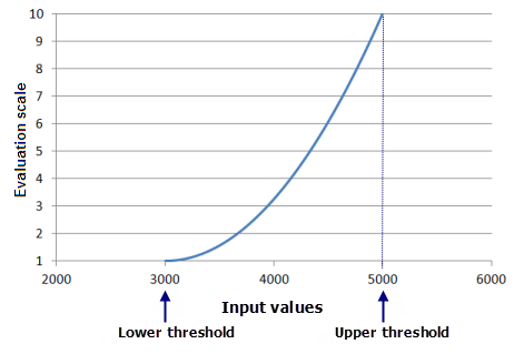
The value range of the input raster is 3,000 to 5,000. All the values in the raster will be transformed using the Power function. The function values, f(x), range from 0 to 4,000,000+ (when applying the shift). This function value range is then rescaled to the defined 1 to 10 evaluation scale with the f(x) of 3,000 being assigned a 1 on the output raster and the f(x) of 5,000 to a 10. In this case, the minimum and maximum input values will be assigned to 1 and 10, respectively, on the output evaluation scale.
Scenario 2
The defined lower and upper thresholds are within the value range of the input raster. The Power function with an exponent of 2 and a shift of 3500 is used as the example function.
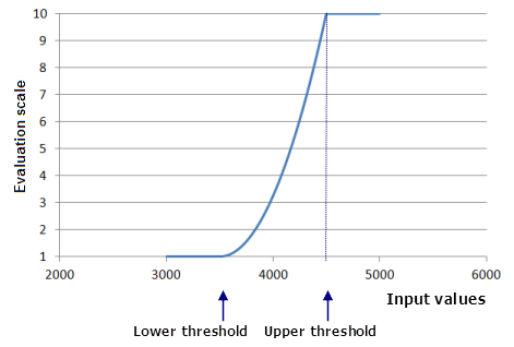
The value range of the input raster is 3,000 to 5,000. The lower threshold is set to 3,500 and the upper threshold to 4,500. The Value below threshold is set to 1 and the Value above threshold is set to 10. The Power function is applied to input values between 3,500 and 4,500. The range of the function values, f(x), (approximately 0 to 1,000,000) are transformed to the 1 to 10 evaluation scale. The cells with an input value of 3,500 (the Lower threshold) will be assigned to 1 and the input values of 4,500 (the Upper threshold) will be assigned to 10 on the output evaluation scale. All values between the thresholds will be assigned to the appropriate evaluation scale value. Notice the minimum and maximum values from the input raster have no effect on the output evaluation scale values. All cells with an input value below 3,500 are assigned 1 and input values above 4,500 will be assigned 10 (the defined values for the below and above threshold parameters); these values are not considered in the function value range.
Scenario 3
The lower or upper thresholds are greater than the input data range. The Power function with an exponent of 2 and a shift of 2,000 is used as the example function.
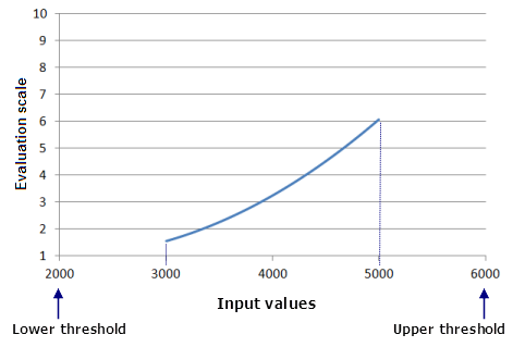
The range of values of the input raster is 3,000 to 5,000. The Lower threshold is set to 2,000 and the upper threshold to 6,000. The Power function will be applied to the values between 2,000 and 6,000. Even though there are no input values equal to 2,000 or 6,000, the function value, f(x), for 2,000 and 6,000 are used to define the lower and upper range of f(x). The function value range is then rescaled to the 1 to 10 evaluation scale. The function value of 2,000 (the Lower threshold) will be assigned a 1 since it will be the lowest f(x) and the function value of 6,000 (the Upper threshold) will be assigned a 10. However, since there are no input values assigned 2,000 or 6,000, there will be no output cells assigned to 1 or 10.
This scenario might be useful when creating a deer habitat suitability model. You may wish the model to reflect the preference of the deer for the locations within the study area relative to the entire deer population in a larger extent. In the study area, the minimum value for the criterion is 3,000 and the maximum 5,000, but for the larger extent encompassing the entire deer population, the minimum value is 2,000 and the maximum value is 6,000.
Scenario 4
The input values map to the lower and upper threshold (the default case) for a function that does not continuously increase or decrease (contains one or multiple peaks). The Gaussian function is used with a midpoint of 4,000 and a spread of 0.00000921 as the example function.
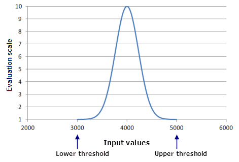
The range of values of the input raster is 3,000 to 5,000. The lower and upper thresholds are set to the minimum and maximum of the input dataset. The Gaussian function is applied to the input values. The resulting function values, f(x), are then placed on the specified 1 to 10 evaluation scale. The function values of the lower and upper thresholds are the lowest f(x) and are assigned to 1 on the output evaluation scale. The f(x) of the midpoint (4,000) is the highest function value and therefore assigned to 10. Note that, in this function, the lower and upper threshold values do not map to 1 and to 10, respectively, on the evaluation scale.
Scenario 5
A special case is scenario 5. The Gaussian function is used with a midpoint of 4,000 and a spread of 0.00000921 as the example function (same as scenario 4).
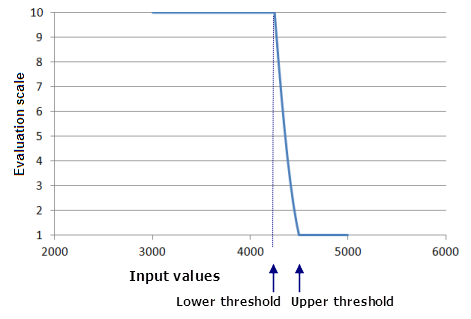
The range of values of the input raster is 3,000 to 5,000. The Value below threshold is set to 10 and the Value above threshold is set to 1. The lower and upper thresholds are set to values to one side of the Gaussian function, to 4,250 and 4,500. The default midpoint and the spread, which are set to the altered thresholds, are overwritten by specified values (to the same as in scenario 4). As a result, the specified Gaussian function (which is not constrained between the thresholds) will be applied only to the input values ranging from 4,250 to 4,500. The function value, f(x), range will be rescaled to the 1 to 10 evaluation scale with the Lower threshold (input value 4,250) being assigned to 10 on the evaluation scale and the Upper threshold (input value 4,500) to 1.