The Rescale by Function tool rescales input raster values based on a specified transformation function. There are a variety of transformation functions and each varies in their calculation and application. Which to use is based on which function best captures the phenomenon being studied. You can further refine the characteristics of each function through a series of input parameters.
In order to get the maximum benefit of the information in this section, it would be helpful to be familiar with the essential vocabulary used for this tool. To understand how the lower and upper thresholds of the transformation function affect the output values see The interaction of the lower and upper thresholds on the output values.
List of functions
The following table provides a summary of each function, with links that will take you to the specific discussion for that function.
Used when the preference increases with an increase in the input values and the preference increases more rapidly as the input values become larger. | |
Used when the highest preferences is around a certain input value with the preferences decreasing as the input values move from the value. | |
Used to indicate that the larger input values have higher preference. | |
Rescales the input values using a linear function. | |
Used when the preference for the lower input values increases rapidly as the values increase and then the preference tapers off with a further increase in the input values. | |
Used when small input values are most preferred. As the values increase the preferences rapidly decrease until the preferences taper off at the larger input values. | |
Used when large input values are most preferred. As the values increase the preferences rapidly increase until the preferences taper off at the larger input values. | |
Rescales input data based on the mean and standard deviation where larger values in the input raster have higher preference. | |
Rescales input data based on the mean and standard deviation where smaller values in the input raster have higher preference. | |
Used when the input values very near the midpoint are more preferred. | |
Used when the preference for the input values increases rapidly with an increase in the input values. | |
Used to indicate that the smaller values from the input raster have higher preference. | |
Used when a particular input value is the most preferred with the preferences decreasing linearly as the input values move from the point. |
Function overviews and illustrations
For each function, a general overview, a use case, and details on the effects of certain input parameters on the function curve will be presented.
Overview
The overview describes the basic properties as well as the specific behaviours for each function.
Use case
The use case describes a specific, real-world example that the particular function may be well suited for.
Effects of the parameters
This section will discuss how the shape-controlling parameters influence the function. It will describe how changing the value for the parameter will influence the curve, and show a graph with several different values for the parameter plotted to illustrate the effects. Also included will be a Python class expression, demonstrating how the transformation function shown in the graphs was constructed.
Note:
For each graph example shown, the input is a raster whose values range between 0 and 500. There is no specific reason for this particular selection, but it is used consistently for all of them to make comparisons easier. In practice, actual input rasters could have any range of input values.
Exponential function
Overview
The Exponential function transforms the input data by applying an exponential function using a specified shift and base factor. In a suitability model, this function is best used when the preference for locations with lower input values are the least preferred, but the preferences increase rapidly for cell locations with larger values.
Use case
Consider how you would rescale the distance from water sources for a tortoise suitability model. Tortoises prefer locations closer to water because of their limited mobility. The preference for locations farther from water quickly decreases as the distance increases.
Effects of the parameters
Input shift
The Input shift is the value subtracted from the input values. The Exponential function is applied to the shifted input values to determine the function values.
Base factor
The Base factor parameter controls how steeply the exponential function increases. As the base factor increases, the preference for the lower input values increases at a slower rate as the input values get larger and then the preference rapidly increases at the larger input values. Altering this parameter may be useful if your input data range is small (for example, 0 to 1) and you want to maintain an exponential curve between the minimum and maximum values.
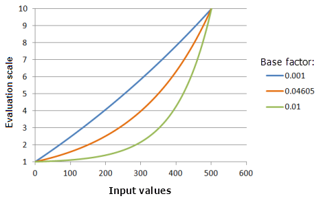
Function used for the graph above:
- TfExponential(0.002651, BaseFactor, 0, 1, 500, 10)
Where the values used for the BaseFactor are: 0.001. 0.04605 and 0.01. The Shift of 0.002651 and the Base factor of 0.04605 are the default calculated parameter values for the input dataset that ranges from 0 to 500.
Gaussian function
Overview
The Gaussian function transforms the input values using a normal distribution. When applying an increasing evaluation scale, the midpoint of the normal distribution defines the most preferred value. If the midpoint is between the lower and upper thresholds, an input value equal to the midpoint is assigned to the To scale value. The remaining input values decrease on the evaluation scale (decrease in preference) as their values move from the midpoint in both directions until they reach the From scale value. In a suitability model, this function is most useful if the highest preference is near a known value with the preferences decreasing as the input values move from the value.
Use case
When installing solar panels, selecting the right direction to have the panels face is important in maximizing their output. For the northern hemisphere, the south-facing aspect (180 degrees) has the highest preference. The preference for the aspects facing more and more toward the east or west continuously decreases, until aspects facing north are the least preferred.
Effects of the parameters
Midpoint
The Midpoint parameter defines the center of the Gaussian curve. You may wish to shift the function midpoint from the data midpoint with either the lower or higher values being more or less important. A second reason you may wish to move the midpoint is to fit the function to values of the criterion outside of the data range.
The midpoint can control the range of the input values the function curve will span.
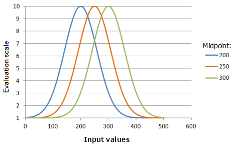
Function used for the graph above:
- TfGaussian(Midpoint, 0.000147, 0, 1, 500, 10)
Where the values used for the Midpoint) are: 200, 250 and 300. The Midpoint of 250 and the Spread of 0.0000147 are the default calculated parameter values for the input dataset that ranges from 0 to 500.
Spread
The Spread parameter controls the steepness of the decay from the midpoint. The greater the value, the narrower the curve becomes around the midpoint (the preference decreases more quickly).
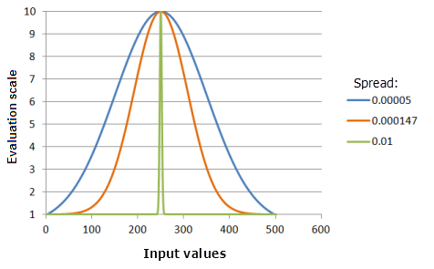
Function used for the graph above:
- TfGaussian(250, Spread, 0, 1, 500, 10)
Where the values used for the Spread are: 0.00005, 0.000147 and 0.01. The Midpoint of 250 and the Spread of 0.0000147 are the default calculated parameter values for the input dataset that ranges from 0 to 500.
Large function
Overview
The Large transformation function is used when the larger input values are more preferred. The defined midpoint identifies the transition point for the function. Values greater than the midpoint increase in preference and values below the midpoint decrease in preference. How quickly the values will increase and decrease as they move from the midpoint is determined by the Spread shape-controlling parameter.
Use case
To create a commodities trading suitability model, you may want to rescale the coffee yield criterion. Locations with higher yield are more preferred, with the preferences increasing nonlinearly with the yield amount.
Effects of the parameters
Midpoint
The Midpoint parameter defines the transition point of the function. Shifting it to be less than the midpoint value of the input data alters the transition point, resulting in an increase in the range of the larger values being more preferred to the right of the midpoint with the preference increasing at a faster rate.
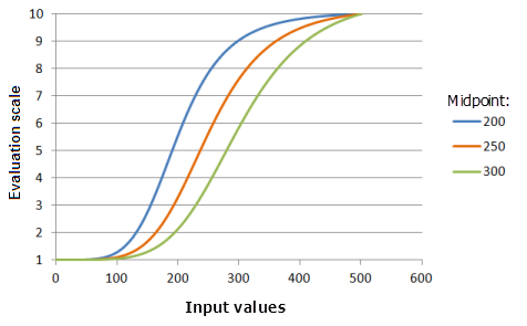
Function used for the graph above:
- TfLarge(Midpoint, 5, 0, 1, 500, 10)
Where the values used for the Midpoint are: 200, 250 and 300. The Midpoint of 250 and the Spread of 5 are the default parameter values for the input dataset that ranges from 0 to 500.
Spread
The Spread parameter controls how quickly the preference increases and decreases. As the spread value increases, input values greater than the midpoint will more quickly increase in preference to the upper threshold, and input values less than the midpoint will more quickly decrease in preference to lower threshold.
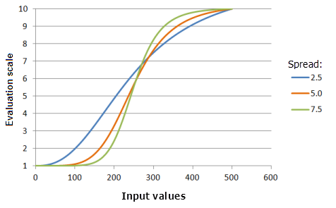
Function used for the graph above:
- TfLarge(250, Spread, 0, 1, 500, 10)
Where the values used for the Spread are: 2.5, 5.0 and 7.5. The Spread of 5 and Midpoint of 250 are the default parameter values for the input dataset that ranges from 0 to 500.
Linear function
Overview
The Linear transformation function applies a linear function between the specified minimum and maximum values. If the From scale is greater than the To scale, a negative linear relationship (a negative slope) is established.
This function is best used when the preferences for values increase or decrease at a constant linear rate.
Use case
To create a climate change suitability model for wildlife habitat, you may need to rescale the wildlife's preference for the elevation values. Within the study area, the larger elevation values are more preferred.
Effects of the parameters
Minimum
The Minimum parameter establishes the first point the Linear function must pass through. You may wish to change the parameter value from the minimum of the input data to correspond to the preference of the phenomenon to the criterion.
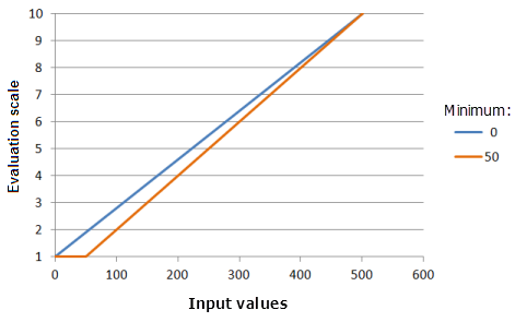
Function used for the graph above:
- TfLinear(Minimum, 500, 0, 1, 500, 10)
Where the values used for the Minimum are: 0 and 50. The Minimum of 0 and the Maximum of 500 are the default parameter values for the input dataset that ranges from 0 to 500.
Maximum
The Maximum parameter establishes the second point the Linear function must pass through. You may wish to change the parameter value from the maximum of the input data to correspond to the preference of the phenomenon to the criterion.
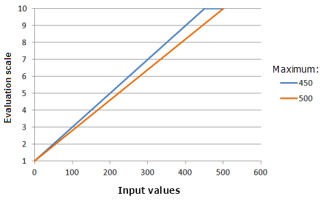
Function used for the graph above:
- TfLinear(0, Maximum, 0, 1, 500, 10)
Where the values used for the Maximum are: 450 and 500. The Minimum of 0 and the Maximum of 500 are the default parameter values for the input dataset that ranges from 0 to 500.
Logarithm function
Overview
The Logarithm transformation function applies a logarithm function to the input data using a specified shift and factor. In a suitability model, the Logarithm function is best used when the preferences increase or decrease rapidly and then taper off with increases in the input criterion values.
Use case
To create a bird suitability model, you may wish to rescale the food quantity criterion. The preference for locations with low amounts of food are the least preferred if they cannot support the birds. When there is enough food for survival, the preference rapidly increases for locations with higher amounts of food since the birds will be more fit. At a certain point, the birds will have enough food so locations with even greater amounts of food will be more desirable but at a much slower rate.
Effects of the parameters
Shift
Shift is the value subtracted from the input values which can control the starting input value for the logarithmic calculations. For example, in the bird use case, if the birds cannot live at locations with less than 250 units of food, you may wish to shift the starting point for the function to 250.
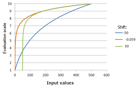
Function used for the graph above:
- TfLogarithm(Shift, 0.0046, 0, 1, 500, 10)
Where the values used for the Shift are: -50.0, -0.059 and 50.0. The Shift of -0.059 and the Exponent of 0.0046 are the default calculated parameter values for the input dataset that ranges from 0 to 500.
Factor
Factor is a multiplier that controls the rise of the logarithm function. You may alter this parameter if the input value range is small (for example, 0 to 1) to maintain a logarithm curve between the minimum and maximum values.
Logistic Decay function
Overview
The Logistic Decay transformation function fits a logistic decay function within a specified minimum and maximum using a defined y intercept percent. In a suitability model, the logistic decay function is best used when the lower input values are more preferred. As the input values increase, the preferences rapidly decrease to a point where the lowest preferences level off at the higher input values.
Use case
To create a housing suitability model, you may want to rescale the distance from electrical lines for the cost of electricity criterion. The locations near existing electrical lines are more preferred because it will cost less to get electricity to them. After a certain distance, the preferences rapidly decrease since additional transformers will need to be installed, incurring additional labor and equipment costs. The decline in preference levels off for the farthest cells since additional cost does not have much additional affect on the preferences since the locations are already too costly.
Effects of the parameters
Minimum
The Minimum parameter controls the starting point of the logistic decay. The greater the minimum value, the faster the preferences will decrease in the main decay portion of the function (the curve will be steeper).
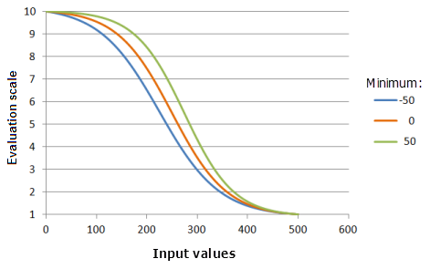
Function used for the graph above:
- TfLogisticDecay(Minimum, 500, 99, 0, 1, 500, 10)
Where the values used for the Minimum are: -50, 0 and 50. The Minimum of 0, the Maximum of 500, and a yInterceptPercent of 99 are the default parameter values for the input dataset that ranges from 0 to 500.
Maximum
The Maximum parameter controls the ending point of the logistic decay. The smaller the maximum value, the faster the preferences will decrease in the main decay portion of the function (the curve will be steeper).
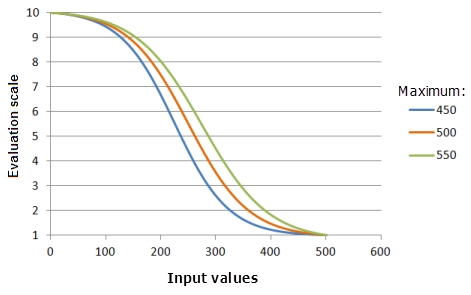
Function used for the graph above:
- TfLogisticDecay(0, Maximum, 99, 0, 1, 500, 10)
Where the values used for the Maximum are: 450, 500 and 550. The Minimum of 0, the Maximum of 500, and a yInterceptPercent of 99 are the default parameter values for the input dataset that ranges from 0 to 500.
Y intercept percent
The Y intercept percent parameter determines the value range that will be in the decay portion of the Logistic Decay curve. Conceptually think of a logistic decay function as a backward "S" shape. There are two tails connected by the main body of the "S", which will be referred to as the decay portion of the curve. The greater the value for this parameter, the input value range included in the decay portion of the curve will be smaller (the "S" is more upright), however, the preference for the values will decrease at a faster rate and the curve will be more pronounced.
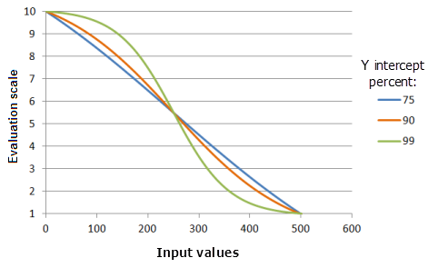
Function used for the graph above:
- TfLogisticDecay(0, 500, YInterceptPercent, 0, 1, 500, 10)
Where the values used for the Y intercept percent are: 75, 90 and 99. The Minimum of 0, the Maximum of 500, and a yInterceptPercent of 99 are the default parameter values for the input dataset that ranges from 0 to 500.
Logistic Growth function
Overview
The Logistic Growth transformation function is similar to the LogisticDecay transformation function, except the preferences in logistic growth function increase instead of decrease.
Use case
In a habitat suitability model, the preferences of an animal increases logistically with the increase in available food. The amount of food first must reach a critical level for survival, then the preference rapidly increases with the increase in food until the maximum intake is reached at which point the preferences level off.
Effects of the parameters
Minimum
The Minimum parameter controls the starting point of the logistic growth. The greater the minimum value, the faster the preferences will increase in the main growth portion of the function (the curve will be steeper).
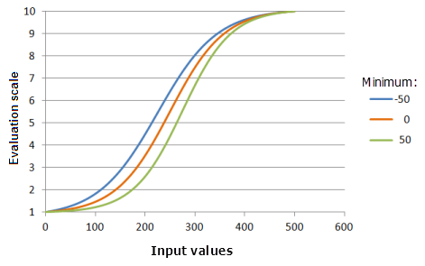
Function used for the graph above:
- TfLogisticGrowth(Minimum, 500, 1, 0, 1, 500, 10)
Where the values used for the Minimum are: -50, 0 and 50. The Minimum of 0, the Maximum of 500, and a yInterceptPercent of 1 are the default parameter values for the input dataset that ranges from 0 to 500.
Maximum
The Maximum parameter controls the ending point of the logistic growth. The smaller the maximum value, the faster the preference will increase in the main growth portion of the function (the curve will be steeper).
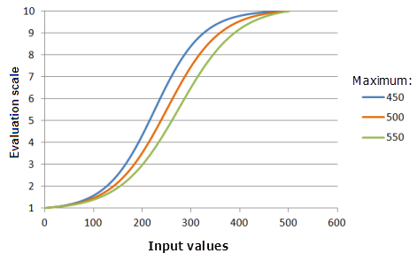
Function used for the graph above:
- TfLogisticGrowth(0, Maximum, 1, 0, 1, 500, 10)
Where the values used for the Maximum are: 450, 500 and 550. The Minimum of 0, the Maximum of 500, and a yInterceptPercent of 1 are the default calculated parameter values for the input dataset that ranges from 0 to 500.
Y intercept percent
The Y intercept percent parameter determines the value range that will be in the growth portion of the Logistic Growth curve. Conceptually think of a logistic growth function as a "S" shape. There are two tails connected by the main body of the "S", which will be referred to as the growth portion of the curve. The smaller the yInterceptPercent, the input value range included in the growth portion of the curve will be smaller (the "S" is more upright), however, the preference for the values will increase at a faster rate and the curve will be more pronounced.
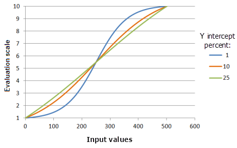
Function used for the graph above:
- TfLogisticGrowth(0, 500, YInterceptPercent, 0, 1, 500, 10)
Where the values used for the Y intercept percent are: 1, 10 and 25. The Minimum of 0, the Maximum of 500, and a yInterceptPercent of 1 are the default parameter values for the input dataset that ranges from 0 to 500.
MSLarge function
Overview
The MSLarge transformation function is similar to the Large transformation function, except the definition of the function is based on specified mean and standard deviation multipliers. Generally, the difference between the two functions is that the MSLarge function can be more applicable if the very large values are more preferred.
The result can be similar to the Large transformation function, given a certain combination of mean and standard deviation multipliers.
Use case
Similar to the commodities trading suitability model discussed in the Large transformation function use case, except the locations with the higher coffee yield are far more preferred in this case.
Effects of the parameters
Mean multiplier
The Mean multiplier parameter controls the slope of the curve of the function. As the multiplier decreases, the favorable range of the larger values increases and, with the larger values, the function curve rises at a slower rate to the upper threshold.
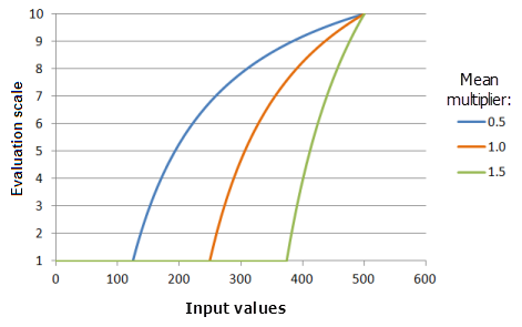
Function used for the graph above:
- TfMSLarge(MeanMultiplier, 1, 0, 1, 500, 10)
Where the values used for the mean are: 0.5, 1.0 and 1.5. The Mean multiplier of 1 and a Standard deviation multiplier of 1 are the default parameter values for the input dataset that ranges from 0 to 500.
Standard deviation multiplier
The Standard deviation multiplier parameter controls the slope of the curve of the function. As the multiplier increases, the function curve increases at a slower rate.
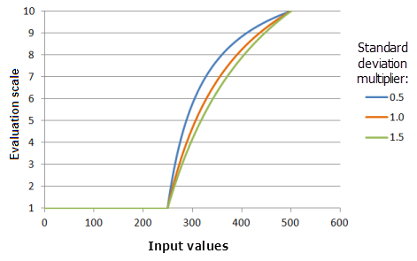
Function used for the graph above:
- TfMSLarge(1, StandardDeviationMultiplier, 0, 1, 500, 10)
Where the values used for the standard deviation are: 0.5, 1.0 and 1.5. The Mean multiplier of 1 and a Standard deviation multiplier of 1 are the default parameter values for the input dataset that ranges from 0 to 500.
MSSmall function
Overview
The MSSmall transformation function is similar to the Small transformation function, except the definition of the function is based on specified mean and standard deviation multipliers. Generally, the difference between the two functions is that the MSSmall function can be more applicable if the very small values are more preferred.
The result can be similar to the Small transformation function, given a certain combination of mean and standard deviation multipliers.
Use case
Similar to rescaling the distance from roads for the cost of construction criterion in the housing suitability model discussed in the Small transformation function, except the closer cell locations are much more preferred in this case.
Effects of the parameters
Mean multiplier
Mean multiplier: controls the slope of the curve of the function. As the multiplier increases, the favorable range of the smaller values increases and, with the larger values, the function curve decreases at a faster rate to the upper threshold.
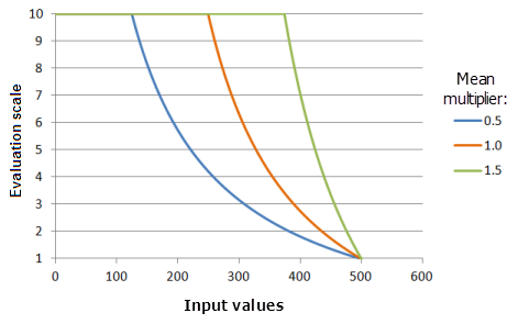
Function used for the graph above:
- TfMSSmall(MeanMultiplier, 1, 0, 1, 500, 10)
Where the values used for the mean are: 0.5, 1.0 and 1.5. The Mean multiplier of 1 and a Standard deviation multiplier of 1 are the default parameter values for the input dataset that ranges from 0 to 500.
Standard deviation multiplier
The Standard deviation multiplier parameter controls the slope of the curve of the function. As the multiplier increases, the function curve decreases at a slower rate.
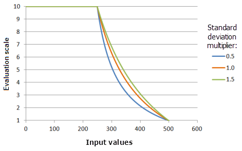
Function used for the graph above:
- TfMSSmall(1, StandardDeviationMultiplier, 0, 1, 500, 10)
Where the values used for the standard deviation are: 0.5, 1.0 and 1.5. The Mean multiplier of 1 and a Standard deviation multiplier of 1 are the default parameter values for the input dataset that ranges from 0 to 500.
Near function
Overview
The Near transformation function is most useful if the highest preference is near a specific value. If the midpoint is between the lower and upper thresholds, an input value equal to the midpoint is assigned to the To scale value. The remaining input values decrease on the evaluation scale (decrease in preference) as their values move from the midpoint in both directions until they reach the From scale value.
The Near and Gaussian transformation functions can be similar, depending on the specified parameters. The Near function generally decreases at a faster rate, with a narrower spread, than the Gaussian function. It is therefore used when the values very near the midpoint are more preferred.
Use case
Similar as the solar panel suitability model discussed in Gaussian transformation function, except the southern aspects are far more preferred.
Effects of the parameters
Midpoint
Midpoint: the same as the midpoint for the Gaussian function, defines the center of the function curve.
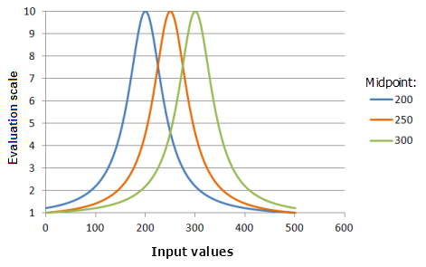
Function used for the graph above:
- TfNear(Midpoint, 0.000576, 0, 1, 500, 10)
Where the values used for the Midpoint are: 200, 250 and 300. The Midpoint of 250 and the Spread of 0.000576 are the default calculated parameter values for the input dataset that ranges from 0 to 500.
Spread
The Spread parameter is similar to the Gaussian function, except with a more dramatic effect as the input values move away from the midpoint.
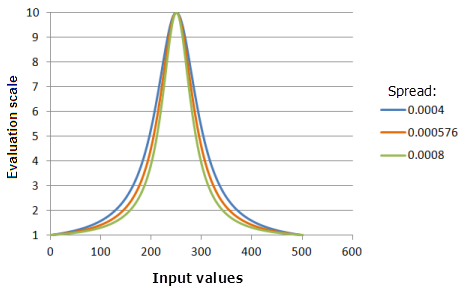
Function used for the graph above:
- TfNear(250, Spread, 0, 1, 500, 10)
Where the values used for the Spread are: 0.0004, 0.000576 and 0.008. The Midpoint of 250 and the Spread of 0.000576 are the default calculated parameter values for the input dataset that ranges from 0 to 500.
Power function
Overview
The Power transformation function applies a power function to the input data raised to a specified exponent using a defined shift. In a suitability model, the Power function is best used when the lowest input values are the least preferable, but as the input values increase the preferences increase until reaching the larger input values where the preferences rapidly increase (this behavior is dependent on the exponent).
Use case
In a suitability model for locating a nuclear power plant to rescale the distance from faults for the safety criterion. Locations farther from a fault line continuously increase in preference based on a power function, that is, locations farther from the fault line are dramatically more preferred than locations closer to the fault.
Effects of the parameters
Shift
The Shift parameter is the value subtracted from the input values which can control the starting input value for the power calculations. For example, in the nuclear power plant use case, it has been determined the plant should not be built within 10 kilometers of the fault line. You may wish to shift the function so that the Power function begins at 10 kilometers.
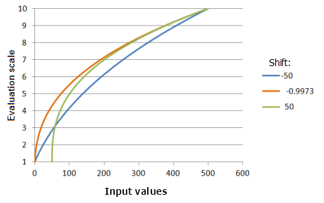
Function used for the graph above:
- TfPower(Shift, 0.3704, 0, 1, 500, 10)
Where the values used for the Shift are: -50.0, -0.9973 and 50.0. The Shift of -0.9973 and the Exponent of 0.3704 are the default calculated parameter values for the input dataset that ranges from 0 to 500.
Exponent
The Exponent parameter controls how steep the Power function increases. The larger the exponent, the steeper the function curve, especially at the larger input values.
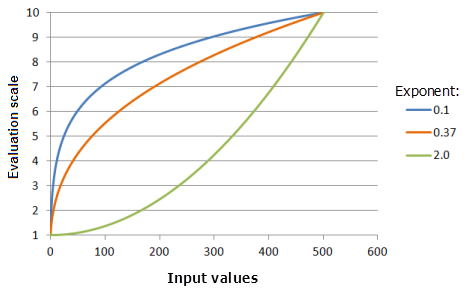
Input parameters for the graph above:
- TfPower(-0.9973, Exponent, 0, 1, 500, 10)
Where the values used for the Exponent are: 0.1, 0.37 and 2.0. The Shift of -0.9973 and the Exponent of 0.3704 are the default calculated parameter values for the input dataset that ranges from 0 to 500.
Small function
Overview
The Small transformation function is used when the smaller input values are more preferred. The defined midpoint identifies the transition point for the function. Values greater than the midpoint decrease in preference and values below the midpoint increase in preference. How quickly the values will increase and decrease as they move from the midpoint is determined by the Spread shape-controlling parameter.
Use case
In a housing suitability model, you may want to rescale the distance to roads dataset for the cost of construction criterion. The locations closer to the roads (the small values) have the highest preference (the lower costs) with the preference values continuously decreasing as the distance from roads increases.
Effects of the parameters
Midpoint
Midpoint: defines the transition point of the function. Shifting the midpoint larger than the midpoint of the input data alters the transition point, resulting in an increase in the range of the smaller values being more preferred to the left of the midpoint with the preference increasing at a slower rate.
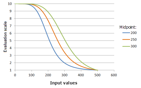
Function used for the graph above:
- TfSmall(Midpoint, 5, 0, 1, 500, 10)
Where the values used for the Midpoint are: 200, 250 and 300. The Midpoint of 250 and the Spread of 5 are the default parameter values for the input dataset that ranges from 0 to 500.
Spread
Spread: controls how quickly the preference decreases and increases. As the spread value increases, input values less than the midpoint will more quickly increase in preference to the lower threshold, and input values greater than the midpoint will more quickly decrease in preference to upper threshold
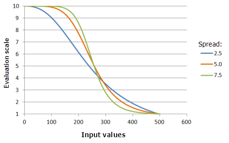
Function used for the graph above:
- TfSmall(250, Spread, 0, 1, 500, 10)
Where the values used for the Spread are: 2.5, 5.0 and 7.5. The Midpoint of 250 and the Spread of 5 are the default parameter values for the input dataset that ranges from 0 to 500.
Symmetric Linear function
Overview
The Symmetric Linear transformation function applies a linear function between the specified minimum and maximum values which is mirrored around the midpoint of the Minimum and Maximum. The corresponding input value to the mirrored point receives the highest preference value, with input values decreasing linearly in preference as they move from the mirrored point. Any input values below the Minimum but above the Lower threshold or above the Maximum but below the Upper threshold will be assigned to the From scale.
If the Minimum is greater than the Maximum, a negative linear relationship (a negative slope) is established.
The Symmetric Linear function is best used when the highest preference is at the midpoint value with the preferences increasing and decreasing linearly as the input values move from the midpoint.
Use case
A particular disease carrying insect is least active at 70 degrees Fahrenheit. As the average temperature increases or decreases toward the minimum and maximum average temperatures within the study site, the insect is more active resulting in more cases of illness in humans. When locating a regional recreation facility, areas with an average temperature of 70 (average temperature) are the most preferred with preference decreasing linearly as temperatures increase and decrease from 70 degrees until reaching the minimum and maximum average temperatures within the study area.
Effects of the parameters
Minimum
The Minimum parameter establishes one of the points the SymmetricLinear function must pass through. Changing the minimum may change the midpoint of where the function is mirrored. You may also wish to change the minimum from the minimum of the input raster to correspond to the preference of the phenomenon to the criterion.
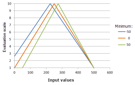
Function used for the graph above:
- TfSymmetricLinear(Minimum, 500, 0, 1, 500, 10)
Where the values used for the Minimum are: -50, 0 and 50. The Minimum of 0 and the Maximum of 500 are the default parameter values for the input dataset that ranges from 0 to 500.
Maximum
Maximum: establishes the second point the SymmetricLinear function must pass through. Changing the maximum may change the midpoint of where the function is mirrored. You may also wish to change the maximum from the maximum of the input raster to correspond to the preference of the phenomenon to the criterion.
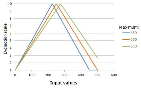
Function used for the graph above:
- TfSymmetricLinear(0, Maximum, 0, 1, 500, 10)
Where the values used for the Maximum are: 450, 500 and 550. The Minimum of 0 and the Maximum of 500 are the default parameter values for the input dataset that ranges from 0 to 500.