Connect locations with corridors

Connecting locations with a path in the most optimal way can be done using the Optimal Region Connections, Optimal Path As Line, and Optimal Path As Raster tools. However, you may want a result that is not limited to a narrow polyline or a one-cell wide path. You want a wider, two-dimensional area where the total cost of travel between locations is less than a particular threshold. This area is called a corridor.

It is possible to produce an area by buffering out an optimal path by a fixed distance. However, this approach may not properly capture what is important to the traveler. For example, a simple buffer around an optimal path might include an industrial park, which would not be suitable to include if you are planning a wildlife corridor. The width of the corridor that will connect the locations should be able to vary in accordance with the rate the actual accumulated cost varies from cell to cell between the locations. Since the industrial park would be a high cost for wildlife, that area would not be included in the corridor.

The corridor encompasses all the possible cost paths that are less than the specified accumulative cost. To define the corridor, the Least Cost Corridor tool sums the per-cell accumulation cost rasters between the sources and selects those cells that are less than the specified cost threshold.

Corridor application examples

Corridors can be used to solve analysis for various scenarios, such as the following:

• In a deer conservation plan, connect two patches of deer habitat with the optimal corridor.
• Identify the possible route for a proposed underground pipeline.
• Determine the feasible area that a proposed bike trail must stay within when connecting two parks.

Corridor analysis

Distance analysis can be divided conceptually into the following related functional areas:

• Calculate straight-line distance and optionally adjust the calculations with a barrier or surface raster.
• Optionally determine the rate the distance will be encountered using a cost surface, source characteristics, vertical factor, and horizontal factor. Create the accumulative distance raster.
• Connect regions over the resulting accumulative distance surface through an optimal network, specific paths, or corridor.

From the third functional area, locations are connected with corridors as illustrated in the examples below.

There is a bear population in a newly established park (light green polygon) and a second population in the surrounding area around one of the four ranger stations (the yellow point). A corridor will allow the bears to move between the two locations.

The final corridor between two locations, a new park and a ranger station (brown area), was created using the Least Cost Corridor tool.

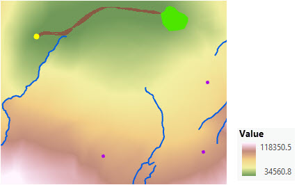
Two accumulative cost distance rasters and two back direction rasters were created with the Distance Accumulation tool using a cost surface, streams as a barriers (blue lines), and a surface raster. The four rasters are entered into the Least Cost Corridor tool and a threshold is specified to define the width of the corridor.

Create a corridor

The general process to identify a corridor between two sources is as follows:

• Calculate the accumulated distance and back direction from the first source location to every other cell in the study area.
• Calculate the accumulated distance and back direction from the second source location to every other cell in the study area.
• Calculate the sum of the accumulated distance between the two sources for each cell.
• Identify the cells whose total accumulated distance between the two sources falls within a defined threshold.

To create a corridor result, complete the following steps:

Calculate the distance accumulation and back direction for the first source.

1. Open the Distance Accumulation tool.
2. Provide the first location to connect as a source (Source 1) in the Input raster or feature source data parameter.
3. Name the output distance raster for Source 1.
4. Identify the cost raster in the Input cost raster parameter.

   The direction of the traveler cannot be incorporated in a corridor. Consequently, do not specify a vertical factor, a horizontal factor, or a value for the Travel Direction source characteristic parameter.

5. Name the output back direction raster.
6. Click Run.
Calculate the distance accumulation and back direction for the second source.
7. Open the Distance Accumulation tool.
8. Provide the second location to connect as a source (Source 2) in the Input raster or feature source data parameter.
9. Name the output distance raster for Source 2.
10. Specify the same parameters as you did in step 4.
11. Name the output back direction raster.
12. Click Run.
Calculate the corridor between the two sources.
13. Open the Least Cost Corridor tool.
14. Identify the output accumulative distance raster for the first location (Source 1) that was created in step 6 as the Input accumulative cost distance raster 1 parameter value.
15. Identify the output back direction raster for the first location (Source 1) that was created in step 6 as the Input back direction raster 1 parameter value.
16. Identify the output accumulative distance raster for the second location (Source 2) that was created in step 12 as the Input accumulative cost distance raster 2 parameter value.
17. Identify the output back direction raster for the second location (Source 2) that was created in step 12 as the Input back direction raster 2 parameter value.
18. Name the output corridor raster.
19. Specify the Threshold method. Select either No threshold, Percent of least cost, or Accumulative cost.
20. If Percent of least cost or Accumulative cost are selected as the Threshold method, specify the percent or accumulative cost threshold that will be used to define the width of the corridor.
21. Click Run.

Connect locations with least-cost corridors

A corridor defines the least-cost geographic area that connects two source locations. It contains all nondirectional cost paths between the sources that are less than a specified accumulative cost. The corridor and paths within it are nondirectional because it does not matter which way you are traveling between the sources.

Corridor creation process

To create a corridor raster, you need four datasets: two that define the distance characteristics to the first source location and another two that define the distance characteristics to the second location. You'll use the Distance Accumulation tool to create an accumulated cost raster and the back direction raster for the first set of sources. Then use the same tool to create an accumulated cost raster and a back direction raster for the second set of locations. Use these two results as input to the Least Cost Corridor tool, which creates a sum of accumulated cost between the two sources and optionally applies a threshold. Only those cells that fall within that threshold are selected to create the final corridor raster result.

Set a threshold

There are three methods for setting a threshold, No threshold, Percent of least cost, and Accumulative cost.

When the No threshold option is specified, the resulting corridor encompasses the full extent of the addition of the two input accumulative cost rasters.

When Percent of least cost is specified, the corridor is created by applying the specified percent to the minimum value in the corridor surface. If a percent of zero, or near zero, is specified, certain cells may become disconnected from the corridor. These cells are connected to the corridor using the input back direction rasters. For additional information, see the Disconnected cells within the corridor section below.

When Accmulative cost is selected and a threshold is specified, all cells with accumulative cost equal to or less than the specified threshold will be selected to create the corridor. The specified threshold value must be equal to or above the minimum value in the corridor surface. If the selected cells do not create a connected corridor between the input sources, they will be connected using the input back direction rasters. For more information, see Disconnected cells within the corridor section below.

Examine the corridor

The image below shows an example of a corridor that was created for a proposed powerline project. The only criteria for assessing cost for the corridor is the land acquisition cost. The final corridor (light red) contains all paths that are at most 10 percent more expensive than the least-cost path derived from the minimum value in the corridor surface, which is also shown (dark red line). The width of the corridor varies along its length, and the corridor diverges noticeably in spots. This result is different than it would be if a fixed width buffer was generated around the least cost path.

The red line shows the least cost path of a proposed powerline. The pink background shows the associated least cost corridor.

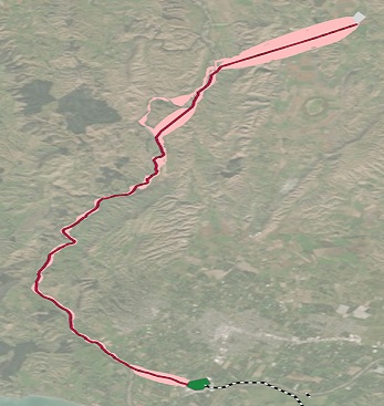
If you select all cells with a total accumulative cost that are at most 10 percent greater than the least-cost path, the result can be considered a 10 percent cost corridor.

Corridor width

Narrow sections of a corridor typically identify areas where the corridor is most sensitive to the costs and there are fewer options for routes through those sections. In the powerline case, the narrower sections of the corridor may be the locations that should be purchased first because there is less latitude where powerlines can be placed in those sections of the corridor. These areas are the most critical locations in the corridor.

When siting wildlife corridors, the narrow sections of the corridor might be where the animals are at most risk when they are moving through the landscape. These narrow areas may be the most important to preserve because wildlife will have fewer options when moving through them.

Another way to visualize the significance of corridor width is to think of a river moving through a valley. Where the valley is wide and flat, there may be many options for the river to pass through that section (taking the least resistance). During a flood, the river can overflow it banks and widen and even follow a different path. However, where the valley narrows into a canyon and has steep walls on both sides, there are few opportunities for the river to change course. The costs surrounding the narrow sections of the canyon can be considered as being much higher. See the Additional information section below for a visual illustration of this concept. In the visualization, the least-cost path is the river and the various cost thresholds are the contour lines.

Appropriate threshold

The threshold is dependent on the units of the cost surface. Cost in dollars is one of the easier units to define. For a wildlife corridor, however, if the cost units are preference, a threshold may be more challenging to determine. Associating a biologic threshold to subjective preference cost units will be more difficult to justify.

In this type of case, several thresholds are tried until the appropriate widths are obtained. Ideally, the specified threshold will be driven by objective measures.

Islands in the corridor

Depending on the specified threshold, islands can be created in the resulting corridor in areas where the corridor diverges and then reconnects, such as in the powerline corridor example above. The island cells have higher accumulative costs, and the corridor will navigate around them.

Corridor directionality

Corridors are nondirectional, so moving from one source to the other has the same cost as moving from the second source back to the first. However, it is important to use the same settings for both runs of the Distance Accumulation tool.

You can use a cost surface and a surface raster to increase the level of complexity in how the distance is being modeled. You cannot, however, use a vertical factor, a horizontal factor, or the travel direction source characteristic since these parameters depend on the directionality of the movement.

Multiple source locations

The number of unique sources that can be used to create the input accumulative cost rasters is not limited to one. Multiple sources can be input to the Distance Accumulation tool. Depending on the accumulative-cost values between the sources and the specified threshold, multiple corridors can be produced between the sources, instead of one single corridor.

Calculate corridors on a per-cell basis

The following diagrams show how a corridor is created for a single cell location. This process occurs for each cell in the input rasters, but for demonstration purposes, one cell will be shown.

To create a corridor, an accumulative cost raster and a back direction raster must be created from source 1 and an accumulative cost raster and a back direction raster be created from source 2 using the Distance Accumulation tool.

The two input accumulative cost rasters are from two sources.

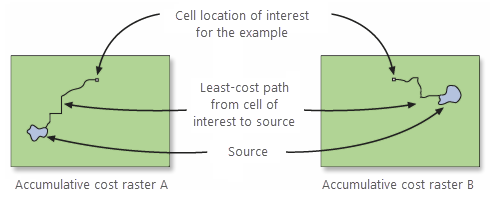
The Least Cost Corridor tool then adds the two accumulative cost surfaces together.

The accumulative cost rasters from two sources are combined.

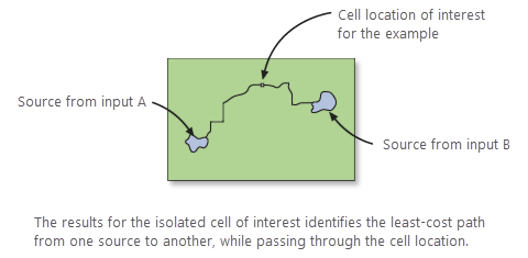
The summed results do not define a single least-cost path between the two sources; it identifies the range of accumulative costs between the sources. That is, the least accumulative cost to reach source 1, plus the least accumulative cost to reach source 2, equals the total accumulative cost of a path passing through a cell. It is the least accumulative cost if a path is routed through the cell between source 1 and source 2.

A threshold is then applied to define the width of the corridor.

All cells with accumulative cost values that are less than the specified threshold are selected from the raster to create a corridor. Once the threshold is applied, the resultant output can be considered the least-cost corridor of cells, not the least-cost path (a single line).

This is the resulting corridor with the threshold applied.

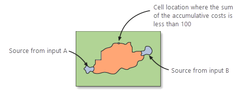
The two back direction rasters are used to ensure there are no disconnected cells in the corridor. For additional information, see Disconnected cells within the corridor section below.

Interpret corridors

The width of a corridor can vary significantly along its length. It is not a fixed distance buffer around a least-cost path. You can define a minimum required width and determine if a set of least-cost paths forms an acceptable corridor.

Another way to think about a corridor is that it shows the uncertainty in the location of a least-cost path. The 10 percent corridor around a given least-cost path is a good visual summary of all paths that are no more than 10 percent more costly than the least-cost path.

A corridor can show where the least-cost path is sensitive to changes in its location. In the powerline example above, the wider area at the top of the corridor is on less expensive land, so there are more options for changing the path’s location in that area without significantly impacting its cost. In contrast, in the narrow middle section of the corridor, the alternative least-cost paths are spatially constricted with few options.

Additional information

The following sections provide additional information regarding connecting locations with corridors.

Cost not Euclidean distance accumulation

There are two main types of distance accumulation raster output from the Distance Accumulation tool: Euclidean or cost distance. The Euclidean distance version of the distance accumulation raster is created when only sources are input. The cost distance version of the distance accumulation raster is most often created from input sources and a cost surface.

If the Euclidean distance version of a distance accumulation raster is input into Least Cost Corridor tool and a threshold is specified, the result will be similar to creating a buffer around the shortest path between the sources. The Least Cost Corridor tool is more effective for the cost distance version of a distance accumulation raster. The width of the corridor is not a simple buffer but is based on cost. Cost distance is the rate that the cost is encountered in each cell. The width of the corridor is therefore based on what is encountered as you move away from the least-cost path.

Disconnected cells within the corridor

Creating a corridor is a two-step analysis.

First, the Distance Accumulation tool calculates the least-cost distance to each cell center in the output accumulative cost raster. To determine the least-cost distance to each cell, a least-cost path is created from the cheapest source to the cell center. The calculation of the path is independent of the raster structure using a numerical calculation method in the Distance Accumulation tool. In the corridor analysis, of particular importance is the ideal least-cost path between source 1 and 2. Since there is no directionality in a corridor, the ideal least-cost path between source 1 and 2 and between 2 and 1 should be the same.

The Distance Accumulation tool maps the ideal least-cost path between the two sources to the cell structure defined by the cost surface or that is set in the Analysis Environment (as well as for all least-cost paths). There is minor distortion in this rasterization process.

The Least Cost Corridor tool takes the sum of the two input accumulative cost rasters and recreates the ideal least cost path between source 1 and 2 from the minimum value in the corridor raster. The derived ideal least-cost path is the basis from which the corridor is determined. The threshold establishes the width of the corridor, which is relative to the derived ideal least-cost path.

Any cell center that falls within the specified threshold will be included in the corridor.

Note:

The derived ideal least-cost path determined by the Least Cost Corridor tool will not always be equal to the realized least-cost path from the Optimal Path As Line tool for the reasons discussed in this section.

A corridor has two requirements:

• It must connect the two input sources.
• All cells in the corridor must be contiguous.

However, there are three factors that can challenge these two requirements:

• Cell size.
• Minor variability in the computations. There is slightly more distortion closer to the sources than farther from them. This minor distortion increases the accumulative cost in those locations and the distortion is slightly compounded when the two input rasters are added together.
• Variability in the cost surface, in particular, in areas with high cost.

As a result of these interacting factors, there are two main scenarios that can create disconnected cells in the corridor. The Least Cost Corridor tool ensures these disconnected cells are connected within the corridor.

Scenario 1

In this scenario, the disconnected cells occur away from the sources where there is less distortion from the variability in the computations and in areas with high-cost cells.

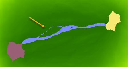
Below is an example of disconnected cells in a wildlife corridor for black bears. The corridor (blue area) connects two habitat patches (purple and yellow areas). The disconnected cells in the middle of the corridor (indicated by the arrow) are in areas of high-cost cells. These disconnected cells will be automatically connected by the Least Cost Corridor tool using the input back direction rasters.

A corridor with disconnected cells between two locations will be connected using the back direction raster in the Least Cost Corridor tool. The cost surface is displayed in the background with darker green being more costly.

The cause of disconnected cells is best illustrated in a simulated example in the image below. The black area is the desired corridor defined by the specified threshold relative to the derived ideal least-cost path irrespective to the cell centers in the corridor map—the sum of the two accumulative costs layers.

The white dots are cell centers, the arrows are the directions to move out of each cell to reach the cheapest source from the back direction rasters, and the gray areas indicate high accumulative cost cells. The corridor breaks happen where accumulative cost cell centers do not fall in the desired corridor area.

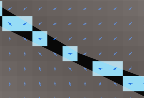
As mentioned earlier, distance accumulation is calculated to each cell center. In areas of high cost, the ideal least-cost path between source 1 and 2 will attempt to limit travel within a high cost cell. However, it may be necessary to pass through part of the cell, such as a corner, avoiding accumulating the full cost to reach the cell center.

The desired corridor defined by the threshold is mapped (rasterized) back to the raster cells of the corridor raster (using the cell center method). Even though the corridor passes through a portion of the high-cost cell, it does not include the cell center. The cell will not be included in the corridor. As a result, certain cells can become disconnected from the corridor.

However, the back-direction input rasters know the way to navigate through these higher cost cells. The Least Cost Corridor tool uses these rasters to connect the disconnected cells to the corridor. The cells that are used to connect these disconnected cells will have a slightly higher accumulative cost than the specified threshold.

To reduce this distortion, a smaller cell size could have been used when creating the distance accumulation rasters in the Distance Accumulation tool. The smaller cell size can capture the actual lower accumulative costs that were aggregated into the coarser cell or it will divide the coarser cell into smaller units. The least-cost path can pass through these smaller cheaper cells, thus avoiding enduring the full cost to reach the center of the cell.

Scenario two

In this scenario, disconnected cells are created when using the Accumulative cost method and setting the threshold close to the minimum value in the corridor surface (the sum of accumulated distance rasters 1 and 2). Alternatively, the Pecent of leat cost method can be used and the percent is set to zero.

In this scenario, the Least Cost Corridor tool derives the ideal least-cost path between the two sources using the minimum value of the sum of the accumulative rasters.

The derived ideal least-cost path passes through the cell or cells with the lowest summed accumulative cost, possibly passing through the cell center. If the least-cost path encounters higher cost areas, the summed accumulative cost for the cells will be greater than the minimum value for the reasons discussed above. Disconnected cells can result. Using the back direction rasters, the Least Cost Corridor tool will make sure the two sources are connected with at least a single cell corridor. All cells used to connect the disconnected cells will have slightly higher accumulative costs than the threshold (the minimum value in the corridor raster).

A generalized version of this scenario is illustrated in the image below. The cost surface is a simulated dataset containing all 1s. The derived least-cost path connecting two sources (pink squares) is shown as a line. The cells that would be selected to include in the corridor using a 0 percent threshold are indicated in black. Since the cost surface contains all 1s, the derived least-cost path is a straight line.

An example is shown of rasterized cell centers being too far away from the derived least-cost path when the set threshold is too close to the minimum value in the corridor raster.

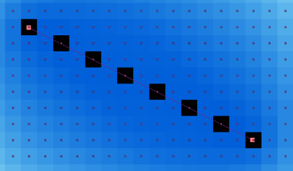
Gaps occur in the corridor (the set of black cells), because the rasterization is too coarse. A connected sequence of cells will not be initially selected. The Least Cost Corridor tool will use the back direction raster to connect the cells creating a continuous corridor.

Understand corridors

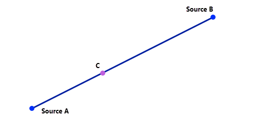
To understand why adding the two distance accumulation rasters and setting a threshold creates a corridor, start with the simplest geometric case. A straight line is the least-cost path between two points in the plane. If point C is on that line, then AC + CB = AB. Using the corridor terminology, the sum of the accumulative costs from C to A and from C to B is constant and is also the minimum (the length of the line AB). As a result, a straight line is the 0 percent corridor between A and B. This is also another way of creating least-cost paths, one where you don’t need a back-direction raster.

Point A and point B are the source points for a line (a least-cost path) and point C is on the line.

If C is moved off the line (away from the least-cost path), AC is the new least-cost path from C to A and CB is the least cost path from C to B. As a result, AC + CB > AB. All points with that same summed cost form an ellipse around the original least-cost path. All least-cost paths connecting C to A and B are contained in the corridor. In corridor terminology, an ellipse is the x percent corridor around the least cost path. As with the powerline example, at the start of the corridor, a least-cost corridor around a least-cost path is different than a fixed width buffer around that path.

Point C is moved from line AB. An ellipse defines a corridor that includes point C.

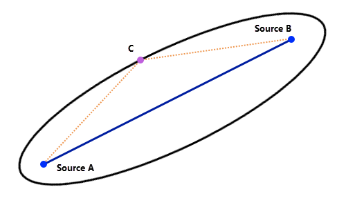
These facts are also true when dealing with more general least cost paths. The 0 percent corridor is identical to the least-cost path and higher threshold corridors form contour loops that contain all cells and all paths in that corridor.

If the direction of motion is not important in your least-cost path analysis, you can use corridors to visualize the uncertainty in the least-cost path or all the locations where alterative nondirectional paths could be located that are within an acceptable cost threshold around the least-cost path.

Visualize corridors

You can gain insight and perspective when viewing corridors in 3D. The least-cost path becomes the relatively level floor of a canyon constructed from the summed accumulative cost input surfaces and the various x percent corridors form contour lines on the canyon walls. From any point on a canyon wall, you must head downhill to get to a source, which means you need to stay below the contour line that indicates you are within that percent’s corridor.

This is a 3D view of the powerline least-cost path and 10 percent corridor. The other contour lines identify potentially more expensive corridors.

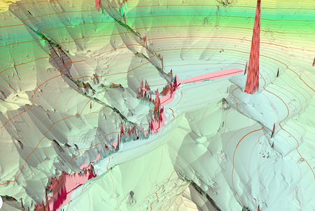
The wider sections of the corridor in the powerline example are contained in the wider, flatter bowl in the image above. If you are willing to spend additional accumulative cost, you can increase the threshold. The wider bowls are where you gain more options for routing the path since the width of the corridor increases significantly. The canyon walls show where that investment will be less successful.