Once the adjusted straight-line distance is calculated, you can use the vertical factor to control the rate at which the distance is encountered. You can use the cost surface, characteristics of the mover, and the horizontal factor to control the rate as well.
The vertical factor accounts for the effort to move through the slopes of the landscape. This effort affects how the distance is encountered. Going uphill may take more effort, going downhill requires less effort, and crossing slopes falls somewhere in between. Modifying the adjusted straight-line distance for this effort helps capture the rate at which distance is encountered by the traveler.

Do not confuse the vertical factor, which represents the effort to overcome slopes, with the surface distance, which is an adjustment to the straight-line distance for the actual distance the traveler covers as they move over the ups and downs in the landscape.
Slope is often relevant to cost distance analysis. Intuitively, it is more costly to overcome steep slopes than flatter slopes. Typically, the Surface Parameters tool is used to generate a slope raster; however, sometimes that slope raster is incorrectly input into the cost surface.
The Slope option in the Surface Parameters tool calculates the rate of change of elevation for each digital elevation model (DEM) cell. It is the first derivative of a DEM. But, as discussed above, it matters how the slope is encountered when moving through a cell. The traveler may avoid a cell assigned a steep slope in a cost surface. This may be effective if the traveler is moving up that slope when traveling through the cell. However, if the traveler is moving down or across that slope when moving through the cell, the cell may be preferred for travel.
You can account for the effort to overcome the slope using the elevation raster in the vertical factor. Do not include the slope raster in the cost surface when the direction that slope is encountered matters.
The direction that slopes are calculated in the vertical factor can also be altered by the Travel direction source characteristic parameter. That is, moving toward or away from a source will change the direction the traveler will enter a cell and as a result, how the slope is encountered.
Incorporating the vertical factor (VF) is a multiplier modifier to the adjusted straight-line distance calculations.
Vertical factor use examples
The vertical factor can be used in various scenarios, such as the following:
- Locate a new hiking trail between two campgrounds that is longer but easier to traverse than hiking directly up the shortest path between them.
- Examine the affects of salt spread on the roads in the winter on the health of the surrounding vegetation. Vegetation downslope from the road will be more impacted by the runoff.
- Determine the movement of a sea creature that is dependent on the change in the concentration of salinity.
Incorporate a vertical factor
Distance analysis can be divided conceptually into the following related functional areas:
- Calculate straight-line distance and optionally adjust the calculations with a barrier or surface raster.
- Once the straight-line distance is calculated, optionally determine the rate the distance will be encountered through a cost surface, source characteristics, a vertical factor, and a horizontal factor. Create the accumulative distance raster.
- Connect regions over the resulting accumulative distance surface using an optimal network, specific paths, or a corridor.
From the second functional area, determine the rate at which the distance will be encountered through a vertical factor as illustrated below. The scenario involves a collection of four forest ranger stations (purple dots), and some rivers (blue lines).
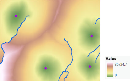
To incorporate the effort for the rangers to overcome the slopes, a vertical factor is specified. The elevation surface is used as the vertical raster.
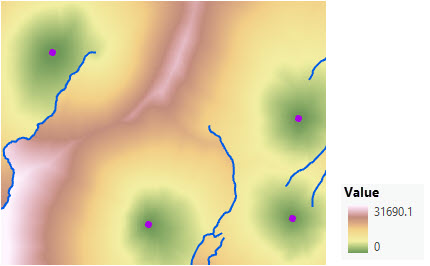
Create a distance raster using a vertical factor
To create a distance map that incorporates a vertical factor, complete the following steps:
- Open the Distance Accumulation tool.
- Provide a source for the Input raster or feature source data parameter.
- Name the output distance accumulation raster.
- Expand the Costs relative to vertical movement category.
- Provide a vertical factor raster for the Input vertical raster parameter.
This input is used to calculate the slope that is encountered when moving between cells. Typically, an elevation raster should be specified.
The Vertical factor parameter appears.
- Specify the settings for the Vertical factor parameter.
This parameter identifies the multiplier to be applied to the cost to adjust for the effort to move through the encountered slopes.
- Click Run.
Vertical factor affects the rate distance is encountered
In order to modify the rate distance is encountered and account for the effort of the traveler to overcome slopes, internally the tool performs two actions:
- Calculate how the slope is encountered when moving from one cell to the next. This is referred to as the vertical relative moving angle (VRMA).
- Identify how the VRMA will modify the rate the distance is encountered.
Calculate the VRMA
The VRMA is the angle of slope from the processing cell (the From cell) to the cell that the traveler is moving into (the To cell). The distance is being calculated for the To cell. The heights from which the slopes are calculated are defined by the input vertical factor raster.
The slope is calculated using the Pythagorean theorem formula of rise/run. The base of the triangle necessary for determining the slope is derived from the adjusted straight-line distance. The height is established by subtracting the From cell value from the To cell value. The resultant angle is the VRMA.
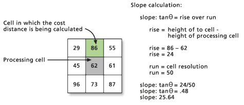
The VRMA is specified in degrees. The range of values for the VRMA is -90 to +90 degrees, accounting for both positive and negative slopes.
Identify the VF multiplier
The VRMA value is then plotted on the specified vertical factor graph to obtain the vertical factor multiplier that will be used in the calculations that determine the cost to reach the To cell. The distance value to move through the cell is multiplied by the identified vertical factor. The larger the vertical factor, the more difficult the movement. A VF greater than 1 increases the cost distance encountered. A VF less than 1 but greater than 0 allows the mover to encounter the distances at a faster rate.
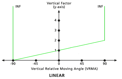
For example, the following graph shows the relationship of the VF and the VRMA for a linear VF function:
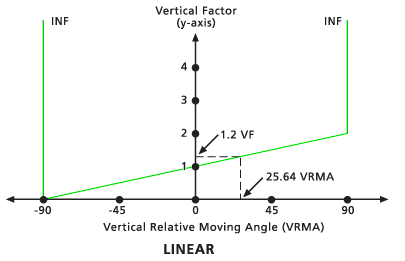
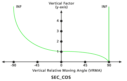
The vertical factor functions that allow you to capture the interaction of the traveler to the slopes they are encountering are Binary, Linear, Inverse linear, Symmetric linear, Symmetric inverse linear, Cos, Sec, Cos-Sec, and Sec-Cos. See the Additional information section below for details of each function.
Note:
The vertical factor is a multiplier. Take care when specifying the units when combining the vertical factor with a cost surface, source characteristics, or a horizontal factor. Generally, when a cost surface is entered, the vertical factor should be a multiplier adjustment of the rate of cost surface units. If time is the unit for the rate of the cost surface, the vertical factor should be a modifier of time. Only one of these factors can define the units for the rate. The other factors are unitless, and their values are multiplier modifiers of the specified units.
Sample applications that use a vertical factor
Sample applications that use a vertical factor are described below.
Create a downslope buffer to understand the effect of winter salt on vegetation
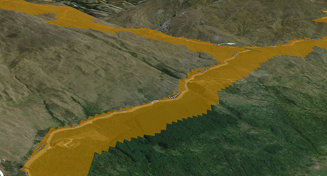
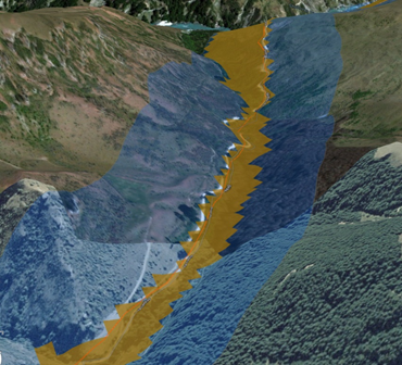
You want to identify areas that are downslope and within 50 meters of a road because these areas may be impacted by winter saltwater runoff. You want to measure the distance along the surface of the terrain. You can use the Binary vertical factor setting to prevent the Distance Accumulation tool from identifying cells that are higher than road cells. Examples of the resulting downslope buffers are shown below.
For comparison, a different section of the road is used to show the difference in the straight-line and downslope-only buffers is shown below.
To create a downslope buffer, complete the following steps:
- Open the Distance Accumulation tool.
- Enter the roads in the Input raster or feature source data parameter.
- Name the Output distance accumulation raster value.
- Expand the Costs relative to vertical movement category.
- Provide an elevation raster in the Input vertical raster parameter.
- Set Binary for the Vertical factor parameter.
- Expand the Characteristics of the source category.
- Set the Maximum accumulation distance parameter to 50 meters.
- Click Run.
Tobler’s hiking function
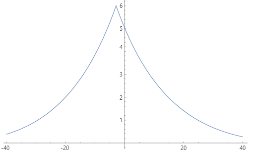
You want to calculate hiking time over the landscape, while adjusting the walking speed based on the slope that is encountered in the direction of travel. Tobler’s hiking function (1993) is an empirical model that is used to perform that adjustment. In the model, it is assumed that a base walking speed is 6 km/h, which is achieved when traveling slightly downslope (about -3 degrees).

Where S is defined in terms of slope d (given in degrees), such that S = tan(d π/180)
The speed function W looks like the following:
You want to know how long it takes to travel a given distance (one cell), not how far you can travel in a specified amount of time, so you need to work with the reciprocal of speed, called pace. The pace in hours per meter (because the horizontal distance analysis units are meters) is expressed, instead of hours per kilometer:

The pace function looks like the following:
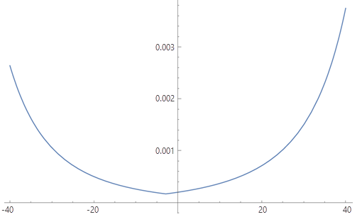
Determine the P(S) for a range of values of d and save them in a table (shown in the Table section below). The table can then be used with the Table vertical factor function to provide a per-cell cost that accounts for the direction of travel through a cell. The cost (in time) to travel through a cell in a specific direction and encountering a slope d is P(S(d)) * cell size (in meters).
To use a nondirectional input cost friction surface in addition to Tobler’s hiking (pace) function in the same analysis, pay attention to the units of cost friction input. At each cell, the Distance Accumulation tool will multiply P(S) * (input cost at the cell), so the values cannot both have units of pace. You can either modify Tobler’s pace function to be solely a weight (replace the 6 with a 1 if you think that is justified empirically), or use unitless weights in your cost input.
Additional information
The following sections provide additional information regarding vertical factors.
Vertical factors
To define the vertical factor function, you can choose one from a list of graphs provided or you can create a custom function using an ASCII file. The following vertical factor functions are available in the Distance Accumulation tool:
Vertical factor options, modifiers, and default values
| Function | Zero factor | Low cut angle | High cut angle | Slope | Power | Cos power | Sec power |
|---|---|---|---|---|---|---|---|
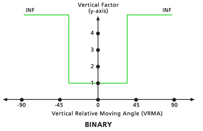
| Binary | 1 | -30 | 30 | N/A | N/A | N/A | N/A |
| Linear | 1 | -90 | 90 | 1.111E-02 | N/A | N/A | N/A |
| Inverse linear | 1 | -45 | 45 | -2.222E-02 | N/A | N/A | N/A |
| Symmetric linear | 1 | -90 | 90 | 1.111E-02 | N/A | N/A | N/A |
| Symmetric inverse linear | 1 | -45 | 45 | -2.222E-02 | N/A | N/A | N/A |
| Cos | N/A | -90 | 90 | N/A | 1 | N/A | N/A |
| Sec | N/A | -90 | 90 | N/A | 1 | N/A | N/A |
| Cos – Sec | N/A | -90 | 90 | N/A | N/A | 1 | 1 |
| Sec – Cos | N/A | -90 | 90 | N/A | N/A | 1 | 1 |
Binary
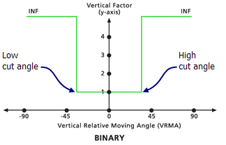
When the VRMA is larger than the low-cutting angle and smaller than the high-cutting angle, the VF for moving between the two cells is set to the value associated with the zero factor. If the VRMA is greater than the cutting angle, the VF is set to infinity. The default cutting angle is 30 degrees if none is specified.
Linear
The VFs are determined by a straight line in the VRMA-VF coordinate system. The line intercepts the y-axis, equitable to the VF factor, at the zero factor value. The slope of the line can be specified using the Slope modifier. If no slope is identified, the default is 1/90 (specified as 0.01111). The default low-cutting angle is -90 degrees, and the default high-cutting angle is 90 degrees.
Inverse linear
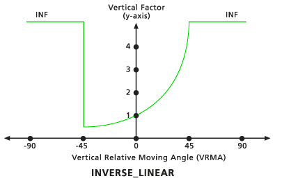
The VFs are determined by the inverse values from a straight line in the VRMA-VF coordinate system. The line intercepts the y-axis, equitable to the VF factor at the zero factor value. The slope of the line can be identified if specified with the Slope modifier. If no slope is identified, the default is -1/45 (specified as 0.02222). The default low-cutting angle is -45 degrees, and the default high-cutting angle is 45.
Symmetric linear
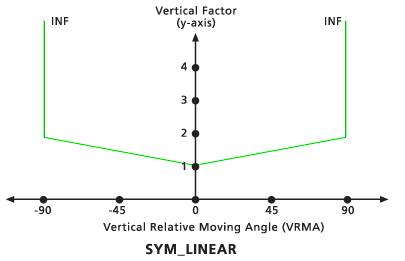
This vertical factor is composed of two linear functions relative to the VRMAs that are symmetrical to the VF (y) axis. Both lines intercept the y-axis at the VF value associated with the zero factor. The slope of the lines is defined as a single slope relative to the positive VRMA using the Slope vertical factor modifier, which mirrors the negative VRMAs. The default slope is 1/90 (specified as 0.01111). The default low-cutting angle is -90, and the default high-cutting angle is 90.
Symmetric inverse linear
This vertical factor is the inverse of the Symmetric linear vertical factor keyword. It is composed of two inverse linear functions relative to the VRMAs that are symmetrical to the VF (y) axis. Both lines intercept the y-axis at the VF value of 1. The slope of the lines is defined as a single slope relative to the positive VRMA using the Slope vertical factor modifier, which mirrors the negative VRMAs. The default slope is -1/45 (specified as 0.02222). The default low-cutting angle is -45, and the default high-cutting angle is 45.
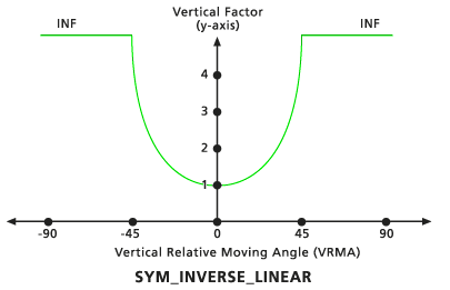
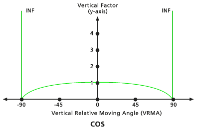
Cos
The VF is determined by the cosine function of the VRMA. The default low-cutting angle is -90 degrees, and the default high-cutting angle is 90 degrees. The default Cos power value is 1.0.
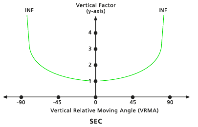
Sec
The VF is determined by the secant function of the VRMA. The default low-cutting angle is -90 degrees, and the default high-cutting angle is 90 degrees. The default Sec power value is 1.0.
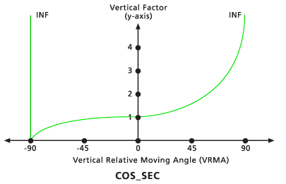
Cos - Sec
When the VRMA is a negative degree value, the VF is determined by the cosine function of the VRMA. If the VRMA is a positive degree value, the VF is determined by the secant function of the VRMA. The default low-cutting angle is -90 degrees, and the default high-cutting angle is 90 degrees. The default Cos power and Sec power values are both 1.0.
Sec - Cos
When the VRMA is a negative degree value, the VF is determined by the secant function of the VRMA. If the VRMA is a positive degree value, the VF is determined by the cosine function of the VRMA. The default low-cutting angle is -90 degrees, and the default high-cutting angle is 90 degrees. The default Sec power and Cos power values are both 1.0.
Table
The table is an ASCII file with two columns on each line.
The first column identifies the VRMA in degrees, and the second column identifies the VF. Each line specifies a point. Two consecutive points produce a line segment in the VRMA-VF coordinate system. The angles must be input in ascending order and range from -90 to 90. The VF factor for any VRMA angle less than the first (lowest) input value or larger than the final (largest) input will be set to infinity. An infinite VF is represented by -1 in the ASCII table.
The following is a sample vertical factor ASCII table. The units of the first column are degrees and the units of the second column are hours per meter.
    -90  -1
    -80  -1
    -70   2.099409721
    -60   0.060064462
    -50   0.009064613
    -40   0.00263818
    -30   0.001055449
    -20   0.000500142
    -10   0.00025934
      0   0.000198541
     10   0.000368021
     20   0.000709735
     30   0.001497754
     40   0.003743755
     50   0.012863298
     60   0.085235529
     70   2.979204206
     80  -1
     90  -1
Vertical factor modifiers
You can further control the VRMA function using modifiers that allow refinement of the vertical factors. There may be a threshold angle such that if the VRMA exceeds it, the cost is so great that it becomes a barrier to travel. This threshold is referred to as the cut angle. The VF is assigned to infinity when the VRMA exceeds this value.
The vertical factor graph will have both lower and upper cut angles in contrast to the horizontal factor graph, which will only have a single cut angle.
Using these modifiers, cut angles can be specified for each of the functions, the trigonometric curves can be raised by a power, the zero factor can alter the y-axis intercept for the nontrigonometric functions, and the slope of the line in the linear functions can be defined.
Zero factor
This modifier establishes the vertical factor used when the VRMA is zero. This factor positions the y-intercept of the specified function.
Low cut angle
This modifier is the VRMA degree that defines the lower threshold, below which (less than) the VFs are set to infinity regardless of the specified vertical factor keywords.
High cut angle
This modifier is the VRMA degree that defines the upper threshold, beyond which (larger than) the VFs are set to infinity regardless of the specified vertical factor keywords.
Slope
This modifier identifies the slope of the straight lines in the VRMA-VF coordinate system for the Linear, Inverse linear, Symmetric linear, and Symmetric inverse linear keywords. Slope is specified as the rise over the run (for example, a 30-degree slope is 1/30 specified as 0.03333). See the Linear VRMA diagram for an example of a linear function with a slope of 1/90.
Power
This modifier is the power to which the values will be raised.
Cos power
This modifier is the power to which the nonnegative values in the Sec-Cos VRMA function and the negative values in the Cos-Sec VRMA function will be raised. The VF is determined by the following:
VF = cos(VRMA)powerSec power
This modifier is the power to which the nonnegative values in the Cos-Sec VRMA function and the negative values in the Sec-Cos VRMA function will be raised. The VF is determined by the following:
VF = sec(VRMA)powerTable name
This modifier identifies the name of the ASCII file that will be used with the Table vertical factor keyword.
References
Tobler, Waldo (1993) Three Presentations on Geographical Analysis and Modeling: Non-Isotropic Geographic Modeling; Speculations on the Geometry of Geography; and Global Spatial Analysis (93-1) Retrieved from https://escholarship.org/uc/item/05r820mz