Choose the best location with Location-Allocation

Available with Network Analyst license.

Location-allocation helps find the best locations for facilities to serve a set of demand locations. The locations may be trying to cover the most amount of demand, minimize costs to reach the demand, or maximize market share. This tutorial shows how to solve for best retail locations to serve customer demand.

Note:

Ensure you are signed in to your ArcGIS Online account. This tutorial can be completed using the network data source as either the designated tutorial network dataset, ArcGIS Online, or an ArcGIS Enterprise routing service published using a network dataset that covers the geography of the input data of the analysis. If you use ArcGIS Online, credits will be consumed.

Learn more about network analysis with a service.

Get the data

The data for this tutorial is available for download.

1. Go to the data download page.
2. Click the Download button, and save the file locally.
3. Unzip the downloaded file.

Create a map

Complete the following steps to create a map:

1. Start ArcGIS Pro.
2. Create a new project by clicking the Map template. Optionally, change the name of your project and location.

   A new project with a map appears.

Add the tutorial data to the project

A network dataset is an intelligent model of the road system. It contains not only the location and attributes of roads, but also information about how roads relate to one another, such as which roads are connected, which turns between connected roads are allowed or prohibited, and other information that affects what travel paths are possible and how long travel takes. The location-allocation solver references the network dataset to determine the cost/distance matrix of shortest paths between facilities and demand locations. The cost/distance matrix is then used to find the best set of locations to which the demand will be allocated.

Note:

If you perform an analysis using ArcGIS Online, the solver references a high-quality, worldwide network dataset stored in the ArcGIS Online cloud and uses ArcGIS Online credits. You can also use your own network dataset stored locally on your machine or use ArcGIS Enterprise to publish routing services using your own network dataset and configure the services with your enterprise portal to consume them from ArcGIS Pro.

In this set of steps, add a network dataset to the map.

1. In the Catalog pane, which is on the right side of the application by default, right-click Folders and choose Add Folder Connection .

   The Add Folder Connection dialog box appears.

2. Browse to the folder where you placed the tutorial data, double-click Network Analyst, and click Tutorial to select the folder.
3. Click OK.

   A connection to the Tutorial folder is created.

Next, add one of the network datasets contained in the folder to the map.

Note:

You do not need to add the network dataset to the map if you intend to use ArcGIS Online or an ArcGIS Enterprise routing service as the network data source.

4. In the Catalog pane, expand Folders > Tutorial > SanFrancisco.gdb > Transportation.
5. Drag Streets_ND, which has a network dataset icon , onto the map.

   The network dataset is added to the Contents pane and to the map.

6. If needed, right-click Streets_ND in the Contents pane and choose Zoom To Layer to view the San Francisco area.

   By default, network datasets built with traffic data show traffic conditions for the current time when they are added to the map. This network dataset includes historical traffic, so you are seeing typical traffic conditions for the current time and day of the week. Not all roads in this network dataset include traffic, so only the ones that do are shown by default.

   The area covered by the network dataset is where you can perform network analyses.

   Viewing the network dataset isn't required to perform an analysis, so next, you will hide it.

7. In the Contents pane, uncheck Streets_ND to display the basemap only.
Add the points that represent candidate stores to the map.
8. In the Catalog pane, browse to Tutorial > SanFrancisco.gdb > Analysis.
9. In the Catalog pane, right-click the CandidateStores layer and choose Add To Current Map.

   The CandidateStores layer is added to the Contents pane and to the map.

Add the points that represent demand to the map.
10. Repeat step 9 to add the following layers to the Contents pane and to the map.
    • TractCentroids
    • ExistingStore
    • CompetitorStores

    Note:

    You can also add a layer to the map by dragging it from the Catalog pane onto the map.

Create the location-allocation layer

A location-allocation layer provides the structure and properties needed to set up and solve the location problem. It also contains the results after solving.

1. On the Analysis tab, in the Workflows group, click Network Analysis > Location-Allocation .

   The location-allocation layer is added to the Contents pane. It includes the sublayers that hold the inputs and outputs of the analysis.

   Location-allocation is referencing the San Francisco network dataset because the network was in the Contents pane when the location-allocation layer was created.

   Note:

   To see or change the network data source that will be used to create the network analysis layer, on the Analysis tab, in the Workflows group, you can click the Network Analysis drop-down menu and look under Network Data Source.

2. In the Contents pane, click Location-Allocation to select the group layer.

   The Location-Allocation Layer tab appears.

3. Click Location-Allocation Layer to see the tab's controls.

   

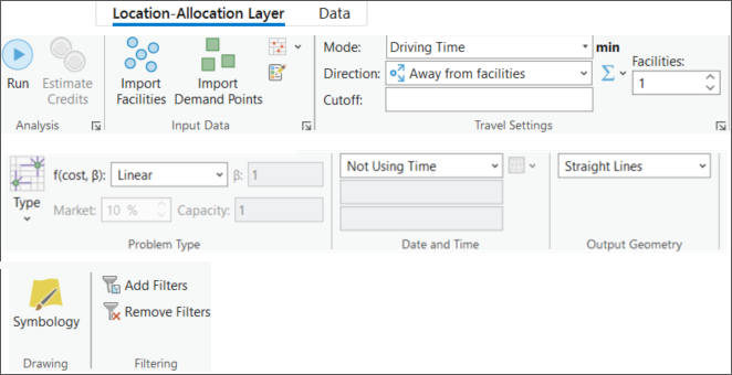
   You'll use these controls to define the location-allocation results you want to generate.

   Tip:

   The Location-Allocation Layer tab appears only when you select a location-allocation layer in the Contents pane. Also, if you have multiple location-allocation layers, you can change the settings of the layers individually or select the multiple layers to edit the settings for all the selected layers if they share the same network data source.

Add candidate facilities

Candidate facilities are the potential places where you can open a store. You'll use the Candidate Stores feature class to add these candidate locations to the network analysis Facilities class. The solution from the location-allocation process will include a subset of these stores.

1. On the Location-Allocation Layer tab, in the Input Data group, click Import Facilities .

   The Add Locations window appears.

2. Make sure Input Network Analysis Layer is set to Location-Allocation and Sub Layer is set to Facilities.
3. Click the drop-down arrow below Input Locations and choose CandidateStores. This is the point feature class you previously added to the map.
4. Leave the default settings for the rest of the parameters and click the OK button.

The 16 candidate stores load as facilities. These locations are drawn on the map with the candidate facility symbol.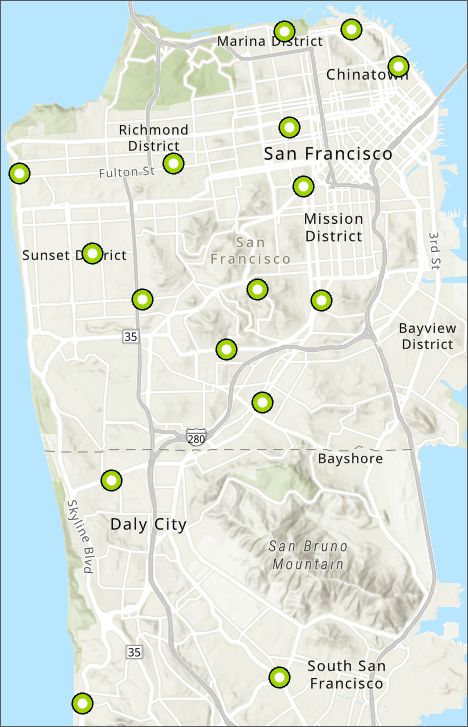

Add demand points

The stores need to be located to best serve the existing population. The Tract centroids point feature class will serve as the demand. The solution from the location-allocation process will allocate these demand locations to the chosen store.

1. On the Location-Allocation Layer tab, in the Input Data group, click Import Demand Points .

   The Add Locations window appears.

2. Make sure Input Network Analysis Layer is set to Location-Allocation and Sub Layer is set to Demand Points.
3. Click the drop-down arrow for Input Locations and choose TractCentroids. This is the point feature class you previously added to the map.
4. From Field Mappings > Property, choose Weight.
5. From the Field Name drop-down list, choose POP2000.
6. Leave the default settings for the rest of the parameters and click the OK button.

The 208 Tract Centroids load as demand and the population at each location is mapped to the weight property for the demand. These locations are drawn on the map with the demand symbol.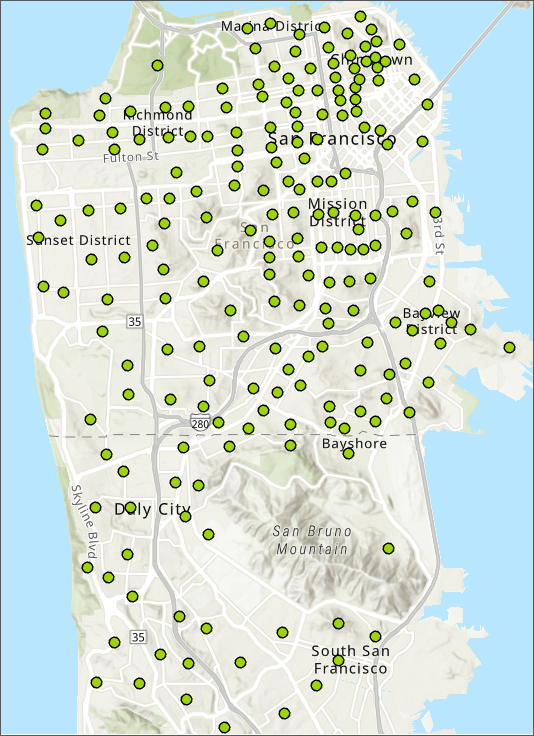

Set up properties of the location-allocation analysis

The Location-Allocation Layer ribbon includes a Problem Type section, where you can specify properties for the locations.

1. On the Location-Allocation Layer tab, in the Problem Type group, click the arrow under Type and choose Maximize Attendance.

   

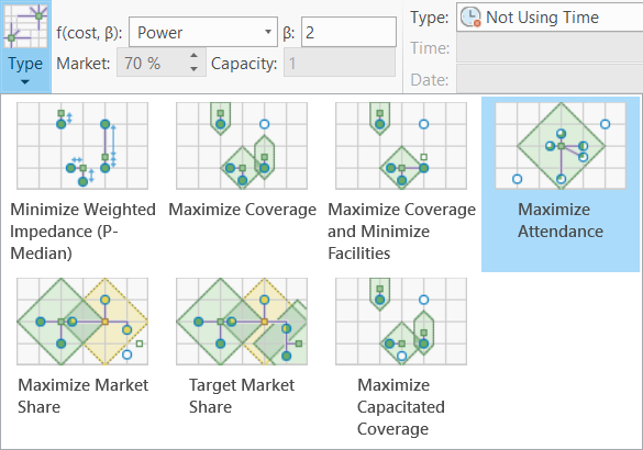
   Maximize attendance is a good problem type for choosing retail store locations. It assumes that all stores are equally attractive and that people are likely to shop at nearby stores.

2. In the Travel settings group, click the Facilities up arrow to 3. This will choose 3 out of the 16 candidate stores to optimally serve the 208 demand points.
3. On the Location-Allocation Layer tab, in the Travel Settings group, in the Cutoff text box, type 5.

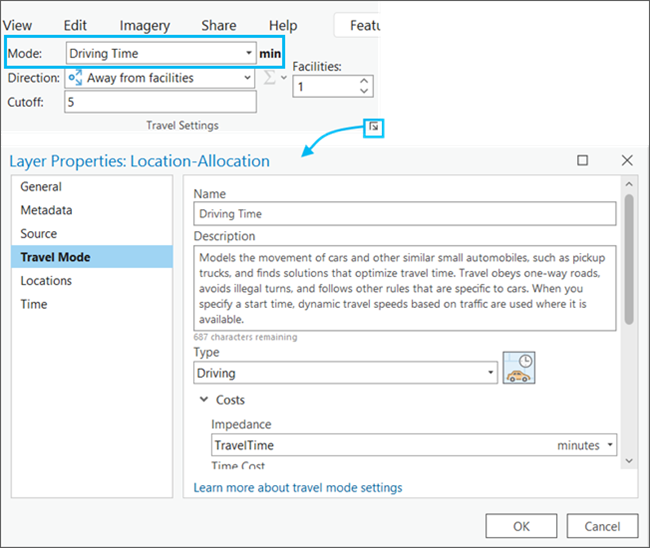
   This implies that people are not willing to travel more than 5 minutes to shop at these stores. The units for this cutoff value are in the units of the current impedance attribute. Since the current impedance is TravelTime, the units are in minutes.

The Driving Time travel mode uses the TravelTime cost attribute, which has units of minutes. Consequently, the Cutoff value is interpreted in units of minutes.

Learn more about the cost attribute

Run the analysis to determine the best store locations

1. On the Location-Allocation Layer tab, click Run .

   The results show the chosen stores connected to the demand they serve with straight lines. These lines also appear in the lines feature class.

Now you'll inspect the results in more detail.
2. In the Contents pane, right-click the Facilities layer and click Attribute Table to open the attribute table.

Examine the attributes of the Facilities table. Three of the features show the FacilityType field values set to Chosen instead of the default status, Candidate.

The DemandCount column lists the number of demand points assigned to each of the chosen facilities. Note that out of the 208 demand points, only 115 were allocated to the chosen facilities because some of the points were farther than the 5-minute cutoff.

The DemandWeight column lists the demand that is allocated to each of the chosen facilities. These values represent the number of people likely to shop at that store.

3. In the Contents pane, right-click the Demand Points layer and click Attribute Table to open the attribute table.

Examine the attributes of the Demand Points table. The FacilityID column has a value of <Null> if the demand point was outside the 5-minute cutoff; however, if a numeric value is present, it represents the ID of the chosen facility to which the demand point was allocated.

The Weight column contains the population count loaded from the census tract feature class. The AllocatedWeight column contains the amount of demand that was apportioned to the associated facility. The amount of weight allocated is based on the linear distance decay and the 5-minute cutoff you set.

Add a required facility

In the previous section, you generated results for where to locate three new stores. In this section, you'll use Location-Allocation to solve a store expansion scenario, in which you'll start with an existing store and optimally locate two additional stores.

1. On the Location-Allocation Layer tab, in the Input Data group, click Import Facilities .

   The Add Locations window appears.

2. Make sure Input Network Analysis Layer is set to Location-Allocation and Sub Layer is set to Facilities.
3. Click the drop-down menu below Input Locations and choose ExistingStore. This is the point feature class you previously added to the map.
4. In the Field Mappings > Property section, choose FacilityType.
5. From the Default Value drop-down menu, choose Required.

   This ensures that when the store is loaded as a facility it will show a status of Required. Required facilities must always be part of the solution.

6. Click the OK button.

Run the process to determine the best store locations with the required facility

1. In the Contents pane, click Location-Allocation to select the group layer.

   The Location-Allocation Layer tab appears.

2. Make sure theLocation-Allocation Layer tab shows the Problem Type to be Maximize Attendance with a 5-minute cutoff and three facilities to locate.
3. On the Location-Allocation Layer tab, click Run .

   When the solve process is complete, lines connect chosen stores to demand points. Note that the original solution changed, and the ExistingStore location is now part of the solution. The other two chosen facilities are now at a different location.

Add competing facilities

Location-allocation can locate new stores to maximize market share in light of competing stores. The market share is computed using a Huff, or gravity, model. A Huff model assumes that demand points have a probability of visiting stores based on some properties of the store as well as the distance away from that store.

1. On the Location-Allocation Layer tab, in the Input Data group, click Import Facilities .

   The Add Locations window appears.

2. Make sure Input Network Analysis Layer is set to Location-Allocation and Sub Layer is set to Facilities.
3. Click the drop-down menu below Input Locations and click CompetitorStores. This is the point feature class you previously added to the map.
4. In the Field Mappings section, click FacilityType, and in the Default Value drop-down menu, choose Competitor.

   This ensures that when the store is loaded as a facility it will have a status of Competitor. Competitor facilities are only used by the Maximize Market Share and the Target Market Share problem types.

5. Click the OK button to finish loading the competitor facilities into the analysis layer.

Set up the properties for maximizing market share with competing facilities

Change the properties of the location-allocation analysis layer so it solves using the Maximize Market Share problem type.

1. In the Contents pane, click Location-Allocation to select the group layer.

   The Location-Allocation Layer tab appears.

2. On the Location-Allocation Layer tab, in the Problem Type group, click the arrow under Type and choose Maximize Market Share. Maximize Market Share computes the probability of customers visiting your facilities as well as competing facilities. It then chooses a set of facilities that maximizes your market share.
3. On the Location-Allocation Layer tab, in the Problem Type group, click the arrow under Cost Transformation Function and change it from Linear to Power. The solver will now use a power decay distance function to determine the propensity to visit the store.
4. Change the Cost Transformation Function Parameter from 1 to 2.

   

   An impedance parameter of 2 on a power impedance transformation means the probability of visiting a store decays with the square of the distance between a demand point and a facility location. Usually, an accurate value of the impedance parameter is computed from other analyses, such as those provided using Esri Business Analyst Online.

Run the process to determine the best store locations while maximizing market share

1. On the Location-Allocation Layer tab, click Run .

   The results show straight lines connecting the demand to the chosen stores as well as the competitor stores. Notice the chosen stores have changed to maximize the amount of demand given the presence of the three competitors.

   The lines overlap more than in the previous solutions, since each demand point in the maximize market share problem can interact with all the facilities that are within the impedance cutoff.

2. In the Contents pane, right-click the Facilities layer and click Attribute Table to open the attribute table.

Examine the attributes of the Facilities table. Three facilities have a FacilityType value of Competitor, one has a value of Required, and two have a value of Chosen, which indicate the solver chose them as the best facilities to open.

The DemandCount column lists the number of demand points assigned to each of the facilities. Note that some demand points were not assigned, since they were outside the 5-minute cutoff.

The DemandWeight column lists the sum of the demand weight assigned to each of the chosen facilities. The weight assigned to your stores versus that assigned to the competitor stores can be used to determine the market share that was reported after the solve process finished.

Achieve a target market share

In the previous section, the three stores chosen accounted for 33.25 percent of the market share. Say, however, you want to capture 70 percent of the market share. You need to know the minimum number of stores that would be needed, and where they should be located, to accomplish that goal. The target market share problem type can help you find the answer.

1. In the Contents pane, click Location-Allocation to select the group layer.

   The Location-Allocation Layer tab appears.

2. On the Location-Allocation Layer tab, in the Problem Type group, click the Type drop-down arrow and change the problem type to Target Market Share.
3. In the Market box, change the default market share from 10% to 70%.
4. On the Location-Allocation Layer tab, click Run .

   The results show straight lines connecting the demand to the chosen stores as well as the competitor stores. Notice there are additional chosen stores in response to the higher market share.

   Open the status message from the previous solve by clicking the Solve History button on the right corner of the Analysis section. It reports that you have achieved 71.06% market share.

   Open the attribute table for Facilities and note that there are now nine chosen facilities in addition to the one required facility. This means you'll need a total of 10 facilities to obtain the 70 percent market share considering the three competitor sites.