The Time Series Cross Correlation tool compares two time series (called the primary and secondary analysis variables) at each location of a space-time cube by calculating a Pearson correlation coefficient between the corresponding values at each time step. Additionally, the secondary analysis variable is time lagged (shifted in time) relative to the primary analysis variable, and new correlations are calculated for various time lags. This allows you to estimate delayed effects between the primary and secondary analysis variables, such as a delay between a marketing campaign and an increase in sales revenue. For example, if marketing and sales are most highly correlated when sales revenue is shifted backward in time by one week, this means that there is a one-week delay between increases in marketing and increases in sales revenue.
The tool can be used as a descriptive and exploratory method to calculate the raw correlation between the time series. It can also be used as an explanatory and inferential method by removing trends and filtering autocorrelation to isolate the statistical dependence between the two variables. You can also include neighbors in the calculations to incorporate similarity between the time series of neighboring locations and capture spatial effects and interactions.
Potential applications
The following are example applications of the tool:
- In a metropolitan area, compare hourly temperatures to electricity usage to prepare for peak electrical demand during the hottest hours of each day.
- Estimate the delay between increases in precipitation levels and increases in reservoir water volume. How long after the peak of a rainstorm do reservoir water levels rise most rapidly? Is the length of the delay different for locations that have different soil conditions?
- Compare the effectiveness of different marketing campaigns to determine which campaign's spending is most positively correlated with sales revenue. Additionally, you can estimate the delay between marketing spending and customer purchases. Do some campaigns take longer to result in sales but ultimately are most effective at generating long-term revenue?
Cross correlation
Cross correlation values measure the strength of the linear relationship between two time series: when one time series increases, does the other tend to increase, decrease, or not change? Cross correlations close to a value of one mean that the two time series move in the same directions and in the same proportions. For example, the number of airline passengers and airline prices are strongly positively correlated: when more people are traveling, airline prices are higher. Similarly, negative cross correlations mean that the two time series move in opposite directions, such as the number of unoccupied parking spaces and the level of street traffic (traffic increases when there are fewer places to park). If two time series are unrelated and do not tend to change in similar or different directions, the cross correlation will be close to zero.
Time lags
Because there are often delayed effects between two time series (for example, the delay between an increase in the number of predators in an ecosystem and changes in the population of the prey), cross correlation values are always calculated with respect to a time lag. The time lag is a shift of the secondary variable relative to the first, and a new cross correlation value is calculated for the new corresponding pairs of values between the two time series.
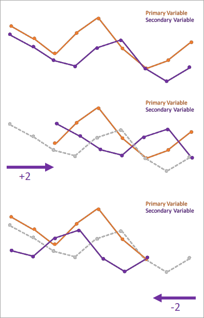
In the image below, the top graph shows the primary and secondary analysis variables. The middle graph shows the secondary variable shifted forward in time two time steps (time lag 2), and the bottom graph shows the secondary variable shifted two time steps backward in time (time lag -2). Because the secondary variable appears to increase or decrease after the primary variable increases or decreases, shifting the secondary variable backward in time (negative time lags) increases the cross correlation between the variables. Also notice that some of the time steps at the ends of the primary variable time series no longer have a paired value in the secondary variable after the shift.

If the time lag with the strongest correlation is positive, changes in the value of the secondary analysis variable occur before changes in the primary analysis variable. Similarly, if the time lag with the strongest correlation is negative, changes in the primary analysis variable occur before changes in the secondary analysis variable.
The tool will calculate cross correlations for all time lags between zero and the value of the Maximum Time Lag parameter. Additionally, the Secondary Variable Lag Direction parameter can be used to specify the direction of the shift (in other words, specify the sign of the time lag). You can shift the secondary analysis variable in both directions, backward in time (negative time lag), or forward in time (positive time lag). For example, using a maximum time lag of 10 and shifting in both directions will calculate cross correlations for all time lags between -10 and 10. Similarly, using a maximum time lag of 5 and shifting only backward in time will calculate cross correlations for all time lags between -5 and 0.
Note:
If no value is provided for the Maximum Time Lag parameter, the maximum time lag will be 10*log10(T/2), for T time steps in each time series (rounded down). The value cannot be larger than (T-5). Providing a value of zero will calculate only the raw cross correlation of the two time series without time lag shifts.
Include spatial neighbors
You can use the Include Spatial Neighbors in Calculations parameter to define a neighborhood around each location to improve the estimate of the cross correlation. If neighbors are included, the cross correlation of each location for a given time lag is the (possibly weighted) average of the cross correlations between the primary analysis variable of the focal location and the time lagged secondary analysis variable of each spatial neighbor (and itself).
For example, in the image below, the focal location is shown in red with eight neighbors around it. The orange time series is the primary analysis variable of the focal location, and the purple time series are the secondary analysis variables at the focal location and at each neighbor. In this case, the cross correlation at the focal location will be the average of nine cross correlations: the cross correlation of the focal feature to itself, the cross correlation of the focal location to the first neighbor, the cross correlation of the focal location to the second neighbor, and so on. In each comparison, the primary analysis variable of the focal location is compared to the secondary variable of the neighbor (or itself). By averaging the correlations, the value better characterizes the cross correlation of the area rather than the individual location. This averaging is repeated for all time lags and all locations.

By default, each correlation is weighted equally in the average, but if you use a distance band or k-nearest-neighbors neighborhood, you can use the Spatial Neighbor Weighting Method parameter to provide larger weights to neighbors that are closer to the focal location. You can use a bisquare or Gaussian kernel to define the weights.
Note:
For distance band neighborhoods, the bandwidth of each kernel is equal to the distance band. See How Kernel Density works to learn how the default distance band is calculated. For k-nearest-neighbors neighborhoods, the bandwidth is equal to the distance to the (k+1)th neighbor. This ensures that all k neighbors are closer than the bandwidth and have nonzero weights. For polygon locations, centroid-to-centroid distances are used to determine neighbors and weights.
Filter and remove trends
For a given time lag, the cross correlation between two time series measures whether the two time series tend to increase and decrease together. This can be considered a descriptive analysis that describes and estimates how strongly the values correspond. However, the raw cross correlation is composed of various factors, including trends, seasonality, autocorrelation, and the statistical dependence of the variables. The raw values of two time series may be highly correlated simply due to shared trends and autocorrelation; for example, sales of ice cream and sunscreen are highly correlated, but if you remove seasonal and economic trends, the correlation becomes very small. You can remove trends, seasonality, and autocorrelation (often called prewhitening and filtering) by checking the Filter and Remove Trends parameter.
Particularly when the goal is to estimate the optimal time lag between the variables, it is important to filter and remove trends. For example, in epidemiological data, there is a time lag between increases in disease counts and increases in hospitalizations. However, using the raw values of the counts frequently shows no time lag between disease and hospitalization due to strong trends and autocorrelation (in other words, time lag zero has the strongest correlation). Instead, when trends are removed and autocorrelation is filtered, the true time lag between disease and hospitalization (for example, 10 days) frequently achieves the strongest correlation.
Because trends, seasonality, and autocorrelation all inflate the type-1 error rate of statistical tests, p-values and 95 percent confidence intervals for the cross correlations are only calculated if you filter and remove trends from the two time series. Additionally, p-values and confidence intervals can only be calculated for pairwise comparisons of two time series. In other words, if you include spatial neighbors in the calculations, p-values and confidence intervals are not calculated for the weighted average of the cross correlations. However, you can use the Output Pairwise Correlations Table parameter to create a table containing p-values and confidence intervals between each location and individual neighbors at all time lags.
Note:
The p-values and confidence intervals are calculated by assuming a normal distribution of the cross correlation with standard deviation equal to the square root of the number of time steps. This is an asymptotic result that is most accurate for time series with at least 30 time steps. A warning will be returned for shorter time series.
The statistical significance tests are independently performed for each time lag of each location, and there is no correction for multiple hypothesis testing. Take caution in interpreting the significance of any particular p-value or confidence interval. All p-values are calculated using two-sided hypothesis tests.
See the Fit a filtering and trend removal model section below for information about how filtering and trend removal is performed.
Tool outputs
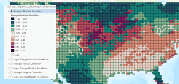
The primary output of the tool is a feature class containing fields of the cross correlation results. In a map, the feature class is added as a group layer containing six layers, each visualizing a different field of the output features. Each layer includes an option to quickly switch between them rather than having to enable and disable each layer individually.
Three of the layers display maps of the strongest correlations: strongest positive correlation, strongest negative correlation, and strongest absolute correlation. Each location is colored by the largest positive correlation, largest negative correlation, or the correlation that is largest in absolute value.

The last three layers show the time lags associated with the three strongest correlation layers. For example, the Lag of Strongest Absolute Correlation layer displays the time lags that resulted in the strongest absolute correlations.

Using these six layers together, you can investigate how strongly correlated the primary analysis variable is to the secondary analysis variable at each location and determine which time lags resulted in these correlations. You may notice spatial patterns in these results; for example, some regions may have smaller time lags or stronger correlations than others. You may also find that the same location can have both a strongly positive and strongly negative cross correlation, depending on the time lag. For example, two time series of a cyclical predator-prey relationship can be made positively or negatively correlated by shifting the cycles of the two time series into or out of alignment.
In addition to the six fields used in the group layer, the output features will have the following fields:
- Object and location ID fields.
- Cross correlation fields for each time lag. A separate field is created for each time lag.
- The number of neighbors of the location. This field is only created if you include spatial neighbors in calculations.
If you filter and remove trends and do not include spatial neighbors in the calculations, the following fields will be created for each of the strongest correlations (positive, negative, and absolute):
- A p-value field testing the statistical significance of the cross correlation.
- Fields of the upper and lower bounds of a 95 percent confidence interval for the cross correlation.
- A binary field (0 or 1) indicating whether the cross correlation is statistically significant (field value 1) or not significant (field value 0) at 95 percent confidence level.
Note:
If all cross correlation values at a location are positive, the strongest negative correlation field and time lag of strongest negative correlation field will contain a null value for that location. Similarly, all negative correlations at a location will produce null values in the strongest positive correlation fields.
The input space-time cube will be updated with the results of the analysis, and you can use the Visualize Space Time Cube in 2D tool with the Time Series Cross Correlation results display theme option to re-create the output feature class and group layer. The analysis variable with the cross correlation results will be the names of the primary and secondary analysis variables with an underscore between. For example, if the input variables are named MARKETING and SALES, the analysis variable with the results will be named MARKETING_SALES.
Pop-up charts
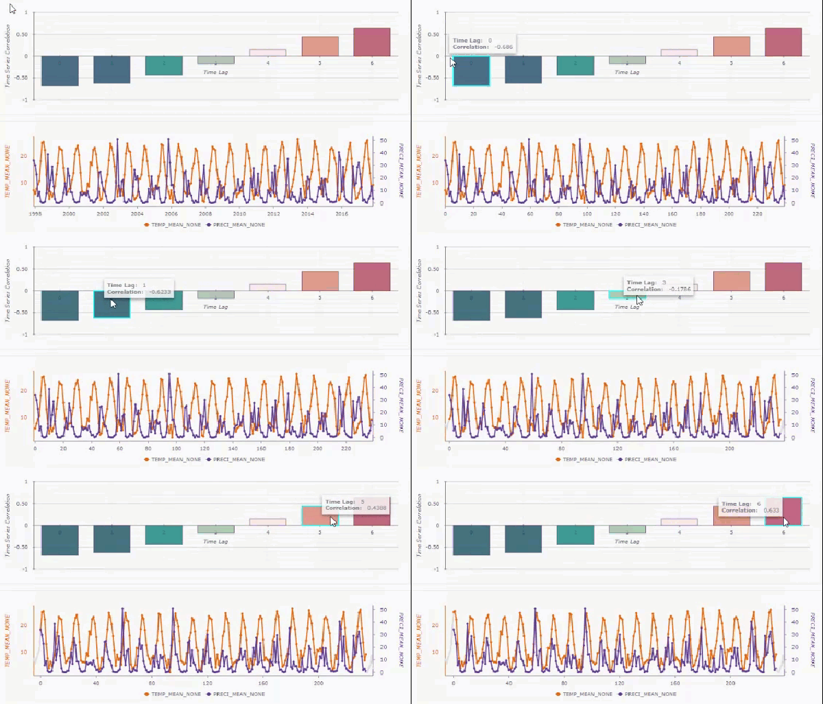
You can create interactive pop-up charts on the output features by checking the Enable Time Series Pop-ups parameter. If created, you can use the Explore tool to click a feature and see a bar chart of the cross correlations for each time lag, along with a line chart showing the primary and secondary analysis variables.

You can hover over any of the bars in the bar chart, and the time series below will shift by the associated time lag. This allows you to see how the two time series align after various time lags.

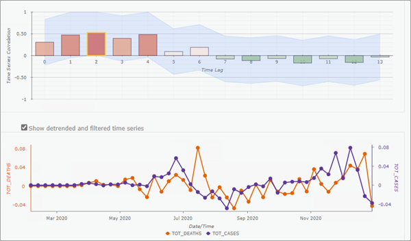
If you filter and remove trends and do not include spatial neighbors, the pop-up chart will display 95 percent confidence intervals (light blue shading) around the cross correlations of each time lag. You can also use the Show detrended and filtered time series check box to display the raw time series values or display the time series after filtering and trend removal.

Note:
If you include spatial neighbors in the calculations, only the time lag bar chart will be displayed. This is to prevent drawing too many time series on each pop-up chart.
Pop-up charts are not created when the output features are saved as a shapefile (.shp).
Output correlation tables
Optionally, you can use the Output Lagged Correlations Table parameter to save the cross correlation results as a table. In the table, each row contains the cross correlation for a single location and a single time lag. The number of rows in the table will be equal to the number of locations multiplied by the number of time lags. Additionally, if you filter and remove trends and do not include spatial neighbors in the calculations, the table will contain fields of the p-value and upper and lower bounds of a 95 percent confidence interval. Saving the information row-wise as a table (rather than as fields of the output features) is often more convenient for exporting and analyzing the cross correlation results. The table can also be joined back to the locations for further analysis.
If you include spatial neighbors in the calculations, you can also use the Output Paired Correlations Table parameter to create a table containing comparisons between each focal location and individual neighbors for every time lag. For example, if there are 10 locations, 5 time lags, and 7 neighbors per location, there will be 10*5*(7+1)=400 rows in the output table (the 1 is added to include the comparisons of the focal location to itself). For each combination, the associated cross correlation is stored as a field. If you filter and remove trends, the table will also contain fields of the p-value and upper and lower bounds of a 95 percent confidence interval.
Geoprocessing messages
The tool provides a number of messages with information about the tool's results. The messages have two sections.
The Input Space Time Cube Details section displays properties of the input space-time cube along with information about the time step interval, number of time steps, number of locations, and number of space-time bins. The properties displayed in this first section depend on how the cube was created, so the information varies from cube to cube.
The Summary of Correlations by Time Lag section displays a table of summary statistics of the cross correlations across all locations for every time lag. For each time lag, the table displays the minimum, maximum, mean, standard deviation, and count of the cross correlations of all locations. If you filter and remove trends and do not include spatial neighbors, the table will also contain a count of locations with statistically significant cross correlations for each time lag. These summary statistics allow you to quickly identify individual time lags that were strongly correlated across many locations, possibly revealing patterns that may not be noticed through exploration of the results of individual locations.
Charts
The three layers displaying the time lags of the strongest correlations (positive, negative, and absolute) each include a bar chart that displays counts of locations that had the strongest correlation for each time lag. For example, in the image below, the majority of locations achieved the strongest absolute correlation with time lag 0, meaning that there is no estimated delay between the two time series at most locations.

Cross correlation formula
For a given time lag, the formula for the cross correlation between two time series is the following:

- k is the time lag.
- t is the time step.
- T is the number of time steps in each time series.
- X(t) is the value of the primary analysis variable at time step t.
- Y(t) is the value of the secondary analysis variable at time step t.
- x̄ is the mean of the primary analysis variable (using all time steps).
- Ȳ is the mean of the secondary analysis variable (using all time steps).
The numerator and denominator are divided by the number of terms in the sums to correct for bias against larger time lags.
Fit a filtering and trend removal model
If you filter and remove trends from the time series, the following preprocessing steps are performed on the primary and secondary analysis variables before time lagging and calculating cross correlations:
- An ordinary least-squares (OLS) regression model is created to predict the next value of the primary analysis variable from the preceding value. In the model, each time step is used as an explanatory variable to predict the value of the next time step.
- A second OLS model is created that predicts the next value of the primary analysis variable from the previous two values. For example, the first two time steps are used to predict the third; the second and third time steps are used to predict the fourth; and so on.
- Three more OLS models are created using three, four, and five previous values, respectively, to predict the next value of the primary analysis variable.
- A fast Fourier transform (FFT) is used to estimate the seasonality of the primary variable, and a sixth OLS model uses this number of time steps to predict the next value.
- AICc values are calculated for each of the six OLS models, and the one with the lowest value is chosen as the filtering and trend removal model.
- Using the coefficients of the chosen model, residuals are calculated for the primary analysis variable, and these residuals become the new primary variable. This step is often called prewhitening the primary variable because the residuals are expected to display random white noise.
- Residuals are calculated for the secondary analysis variable by applying the coefficients to the values of the secondary variable, and these residuals become the new secondary variable. This step is often called filtering the secondary variable. Because the coefficients were estimated from the primary variable, the residuals of the secondary variable are still expected to contain some trends and autocorrelation (rather than random white noise).
- This process is repeated independently for each location. If spatial neighbors are used, the process is performed on the primary variable of the focal location and the secondary variable of each neighbor (and itself).
Note:
The filtering and trend removal process will reduce the length of each time series by the number of time steps used as explanatory variables in the OLS model chosen in step 5. For example, if three time steps are used to predict the next value, residuals cannot be calculated for the first three time steps of each time series.
References
Brockwell, P. J., and Davis, R. A. (2002). Introduction to Time Series and Forecasting. New York, NY: Springer New York. https://doi.org/10.1007/978-3-319-29854-2.
Chan, K.S. and Cryer, J.D. (2008). Time Series Analysis With Applications in R. New York, NY: Springer New York. https://doi.org/10.1007/978-0-387-75959-3.
