How Block Statistics works

The Block Statistics tool performs an operation that calculates a statistic for input cells within a fixed set of nonoverlapping windows or neighborhoods. The statistic (for example, mean, maximum, or sum) is calculated for all input cells contained within each neighborhood. The resulting value for an individual neighborhood or block is assigned to all cell locations contained in the minimum bounding rectangle of the specified neighborhood.

Neighborhood processing

Conceptually, for each block of cells, the algorithm calculates a statistic for the input cells that fall within the specified neighborhood shape in that block. Since the neighborhoods do not overlap, any specific input cell will be included in the calculations for one block only.

Several predefined neighborhood shapes are available to choose from. You can also create a custom shape. The statistics that you can calculate for a neighborhood are majority, maximum, mean, median, minimum, minority, range, standard deviation, sum, and variety.

The Block Statistics tool works as follows:

• It creates the first specified neighborhood—for example, a circular neighborhood—in the upper left corner of the analysis window.

  

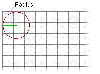
• It calculates the minimum bounding rectangle to determine the size of the output block.

  

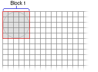
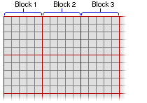
• It partitions the remaining area of the raster into defined blocks. Blocks cannot overlap.

  

• It identifies in each block the cell locations that will be used in the block calculations. The cell locations are determined by the definition of the specified neighborhood—for example, a circular neighborhood—that fits into the bounding rectangle.

  

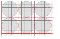
• It calculates the output value for each neighborhood of each block. The resultant values are assigned to every cell location in the corresponding output block.

NoData cells

The Ignore NoData in calculations parameter controls how NoData cells within the neighborhood window are processed. When this parameter is checked (ignore_nodata = "DATA" in Python), any cells in the neighborhood that are NoData will be ignored in the calculation of the output value for the block. When unchecked (ignore_nodata = "NODATA" in Python), if any cell in the neighborhood is NoData, all of the cells in the output block will be NoData.

Neighborhood size

The maximum size of any dimension of a neighborhood is limited to 2,047 cells. This means that rectangular neighborhoods cannot exceed this number of cells in either the horizontal or vertical direction. For circular neighborhoods, the radius cannot exceed 1,023 cells.

Neighborhood types

The shape of a neighborhood can be an annulus (a donut), a circle, a rectangle, or a wedge. Using a kernel file, you can also define a custom neighborhood shape, as well as assign different weights to specific cells in the neighborhood before the statistic is calculated.

Following are descriptions of the neighborhood shapes and how they are defined:

• Annulus
  • The annulus shape is composed of two circles, one inside the other to make a donut shape. Cells with centers that fall outside the radius of the smaller circle but inside the radius of the larger circle will be included in processing the neighborhood. The area that falls between the two circles constitutes the annulus neighborhood.
  • The radius is identified in cells or map units, measured perpendicular to the x- or y-axis. When the radii are specified in map units, they are converted to radii in cell units. The resulting radii in cell units produce an area that most closely represents the area calculated using the original radii in map units. Any cell center encompassed by the annulus will be included in the processing of the neighborhood.
  • The default annulus neighborhood is an inner radius of one cell and an outer radius of three cells.
  • An example illustration of an annulus neighborhood follows:

  

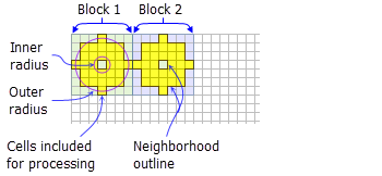
  Two processing blocks are shown with the default annulus neighborhood (inner radius = 1 cell, outer radius = 3 cells).

• Circle
  • A circle neighborhood is created by specifying a radius value.
  • The radius is identified in cell or map units, measured perpendicular to the x- or y-axis. When the radius is specified in map units, additional logic is used to determine which cells are included in the processing neighborhood. First, the exact area of a circle defined by the specified radius value is calculated. Next, the area is calculated for two additional circles, one with the specified radius value rounded down and one with the specified radius value rounded up. These two areas are compared to the result from the specified radius, and the radius of the area that is closest will be used in the operation.
  • The default circle neighborhood radius is three cells.
  • An example illustration of a circle neighborhood follows:

  

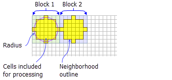
  Two processing blocks are shown with the default circle neighborhood (radius = 3 cells).

• Rectangle
  • The rectangle neighborhood is specified by providing a width and a height in either cells or map units.
  • Only the cells with centers that fall within the defined object are processed as part of the rectangle neighborhood.
  • The default rectangle neighborhood is a square with a height and width of three cells.
  • An example illustration of a rectangle neighborhood follows:

  

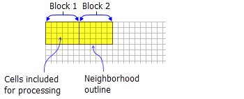
  Two processing blocks are shown with a rectangle neighborhood (width = 6 cells, height = 4 cells).

• Wedge
  • A wedge is a pie-shaped neighborhood specified by a radius, a starting angle, and an ending angle.
  • The wedge extends counterclockwise from the starting angle to the ending angle. Angles are specified in arithmetic degrees from 0 to 360, where 0 is on the positive x-axis (3:00 on a clock), and can be integer or floating point. Negative angles can be used.
  • The radius is identified in cells or map units, measured perpendicular to the x- or y-axis. When the radius is specified in map units, it is converted to a radius in cell units. The resulting radius in cell units produces an area that most closely represents the area calculated using the original radius in map units. Any cell center encompassed by the wedge will be included in the processing of the neighborhood.
  • The default wedge neighborhood is from 0 to 90 degrees, with a radius of three cells.
  • An example illustration of a wedge neighborhood follows:

  

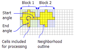
  Two processing blocks are shown with the wedge neighborhood (radius = 3 cells, start angle = 0, end angle = 270).

• Irregular
  • Allows you to specify an irregularly shaped neighborhood.
  • The irregular kernel file specifies the cell positions to be included within the neighborhood.
  • The following apply to a kernel file for an irregular neighborhood:
    • The irregular kernel file is an ASCII text file that defines the values and shape of an irregular neighborhood. The file can be created with any plain text editor. It must have a .txt file extension and no spaces in the file name.
    • The first line specifies the width and height of the neighborhood (the number of cells in the x direction, followed by a space, and the number of cells in the y direction).
    • The subsequent lines define the value to use for each position in the neighborhood they represent. A space between each value is necessary.
    • The values define whether a position in the neighborhood will be included in the calculation. Typically, the value 1 is used to identify the positions to include in the calculations for an irregular neighbourhood, but any positive or negative value other than 0 can be used. Floating point values can also be used.
    • To exclude a location in the neighborhood from the calculation, use a value of 0 (not a blank space) at the corresponding location in the kernel file.

  • The following example shows the contents of an irregular kernel file and the neighborhood it represents:

  

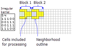
  An irregular neighborhood kernel is shown with an illustration of which cells will be included for processing for two blocks.

• Weight
  • Similar to the irregular neighborhood type, the weight neighborhood allows you to define an irregular neighborhood, but also allows you to apply weights to the input values.
  • The weight kernel file specifies the cell positions to include within the neighborhood and the weights by which they will be multiplied.
  • The weight neighborhood is only available for the mean, standard deviation, and sum statistics types.
  • The following apply to the kernel file for a weight neighborhood:
    • The weight kernel file is an ASCII text file that defines the values and shape of a weight neighborhood. The file can be created with any plain text editor. It must have a .txt file extension and no spaces in the file name.
    • The first line specifies the width and height of the neighborhood (the number of cells in the x direction, followed by a space, and the number of cells in the y direction).
    • The subsequent lines define the value to use for each position in the neighborhood they represent. A space between each value is necessary.
    • For the sum statistic, a weight can be any positive, negative, integer, or floating point value.
    • For the mean and standard deviation statistics, a weight can be any positive integer or floating point value. Negative values are not allowed for these statistics, so any position with a negative weight will be ignored in the calculations.
    • To exclude a location in the neighborhood from the calculation, use a value of 0 (not a blank space) at the corresponding location in the kernel file.

  • The following example shows the contents of a weight kernel file and the neighborhood it represents:

  

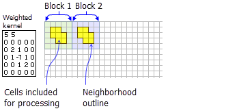
  A weighted neighborhood kernel is shown with an illustration of the cells that will be included for processing for two blocks.

Statistics type

The available statistics are majority, maximum, mean, median, minimum, minority, range, standard deviation, sum, and variety. The default statistics type is mean.

Certain statistics types are only available when the input raster is of integer type.

• Majority
  • Only an integer raster can be used as input.
  • The frequency of each unique cell value in each block neighborhood is determined. If there is a single value that has the highest frequency (occurs the most often), that value is assigned to all cells in that neighborhood. If there is a tie, the lowest of the tied values is assigned.
• Maximum
  • If the input raster is integer, the values on the output raster will be integer; if the values on the input are floating point, the values on the output will be floating point.
• Mean
  • The input can be an integer or a float raster.
  • The output raster will always be floating point.
  • For the weight neighborhood type, this is one of the subset of statistics types that is supported. See the Weighted neighborhood section for details on how this statistic is calculated.
• Median
  • Only an integer raster can be used as input.
  • When the number of valid cell values in the neighborhood is odd, the median value is calculated by ranking the values and selecting the middle value. If the number of values in a neighborhood is even, the values are ranked and from the two middle values, the lower one is selected.
• Minimum
  • If the input raster is integer, the values on the output raster will be integer; if the values on the input are floating point, the values on the output will be floating point.
• Minority
  • Only an integer raster can be used as input.
  • The frequency of each unique cell value in each block neighborhood is determined. If there is a single value that has the lowest frequency (occurs the least often), that value is assigned to all cells in that neighborhood. If there is a tie, the lowest of the tied values is assigned.
• Range
  • If the input raster is integer, the values on the output raster will be integer; if the values on the input are floating point, the values on the output will be floating point.
  • The values for each cell location on the output raster are determined on a cell-by-cell basis by applying this simple formula: Block Range = Block Maximum – Block Minimum.
• Standard deviation
  • The output raster will always be floating point.
  • For the weight neighborhood type, this is one of the subset of statistics types that is supported. See the Weighted neighborhood section for details on how this statistic is calculated.
  • The standard deviation is calculated on the entire population (the N method); it is not estimated based on a sample (the N-1 method).
• Sum
  • If the input raster is integer, the values on the output raster will be integer; if the values on the input are floating point, the values on the output will be floating point.
  • For the weight neighborhood type, this is one of the subset of statistics types that is supported. See the Weighted neighborhood section for details on how this statistic is calculated.
• Variety
  • Only an integer raster can be used as input.

Weighted neighborhood calculations

The amount of influence that each value in the neighborhood has on the final result for the processing block can be adjusted by applying weights.

In the following sections, the formulas used to calculate the results for the weighted mean, standard deviation, and sum statistics are shown. An example accompanies each, showing the calculations for a processing block and the results for a 3 x 3 cell rectangle neighborhood.

Weighted mean statistic

For the weight neighborhood with the mean statistic, the output value for the cells in a processing block is the sum of the product of the kernel weight values multiplied by the input values, divided by the sum of the kernel weight values.

The formula applied to the cells within a neighborhood is as follows:

Where:

• µ_W is the population weighted mean value for the processing block.
• N is the number of cells in the neighborhood.
• w_i is a weight value defined in the kernel.
• x_i is an input cell value.

Legacy:

In previous releases, the calculations used the number of cells in the neighborhood as the denominator.

Weight values must be positive values and can be integer or floating point.

Example

Consider the following 3 x 3 rectangle block of input cells:

4 6 7
6 7 8
4 5 6

The mathematical average (sum / count) of these values is 53 / 9 = 5.889.

Consider the following 3 x 3 weighted cell kernel:

3 3
0.0 0.5 0.0 
0.5 2.0 0.5 
0.0 0.5 0.0

This kernel gives the highest degree of influence to the center cell in the block (weight of 2), lessens the influence of the four orthogonal neighbors to the center cell (weight of 0.5), and makes the four corner cells have no influence (weight of 0).

Applying the weighted mean equation provided above, the following shows the calculations for achieving the final value.

= (w1x1 + w2x2 + w3x3 + w4x4 + w5x5 + w6x6 + w7x7 + w8x8 + w9x9) /
  (w1 + w2 + w3 + w4 + w5 + w6 + w7 + w8 + w9)
= ((0*4)+(0.5*6)+(0*7)+(0.5*6)+(2.0*7)+(0.5*8)+(0*4)+(0.5*5)+(0*6)) /
  (0+0.5 + 0 + 0.5 + 2.0 + 0.5 + 0 + 0.5 + 0)
= (0 + 3.0 + 0 + 3.0 + 14.0 + 4.0 + 0 + 2.5 + 0) / 
  (0.5 + 0.5 + 2.0 + 0.5 + 0.5)
= (3.0 + 3.0 + 14.0 + 4.0 + 2.5) / 4.0
= 26.5 / 4.0
= 6.625

For comparison, the regular average of the nine input cells would be 5.889. If only the five input cells that are within the kernel (where the weight != 0) are included but with the values of the weights not considered, the average would be 6.4 (6 + 6 + 7 + 8 + 5 = 32, which when be divided by the count of five).

Weighted standard deviation statistic

For the weight neighborhood with the standard deviation statistic, the output value for the cells in a processing block is the result of the following equation:

Where:

• SD_W is the population weighted standard deviation value for the processing block.
• µ_W is the population weighted mean value for the processing block.
• N is the number of cells in the neighborhood.
• w_i is a weight value defined in the kernel.
• x_i is an input cell value.

Weight values must be positive values and can be integer or floating point.

If all the input values in a neighborhood are the same, the standard deviation value for all cells in a processing block will be 0.

Example

The same neighborhood values that were used in the weighted mean example above will be used again for this example.

4 6 7
6 7 8
4 5 6

The same weighted kernel values will also be used:

3 3
0.0 0.5 0.0 
0.5 2.0 0.5 
0.0 0.5 0.0

Applying the weighted standard deviation equation provided above for the block of cells, the result of the calculation is approximately 0.85696. This value will be written to every cell in this block neighborhood.

Weighted sum statistic

For the weight neighborhood with the sum statistic, the output value for the cells in a processing block is the result of the following equation:

Where:

• S_W is the weighted sum value for the processing block.
• N is the number of cells in the neighborhood.
• w_i is a weight value defined in the kernel.
• x_i is an input cell value.

Weight values can be positive or negative values and can be integer or floating point.

Example

Consider the following neighborhood input values:

4 6 7
6 7 8
4 5 6

Consider the following 3 x 3 weighted cell kernel:

3 3
-1 -2 -1
 0  0  0
 1  2  1

Applying the equation provided above, the following shows the calculations used to achieve the final value:

= (w1x1 + w2x2 + w3x3 + w4x4 + w5x5 + w6x6 + w7x7 + w8x8 + w9x9)
= ((-1*4) + (-2*6) + (-1*7) + (0*6) + (0*7) + (0*8) + (1*4) + (2*5) + (1*6))
= (-4) + (-12) + (-7) + 4 + 10 + 6
= -3

Uses for block statistics

The Block Statistics tool can be used instead of the Resample tool to resample a raster from a fine resolution to a coarser one. Instead of using the nearest neighbor, bilinear, or cubic resampling techniques, it may be preferable to assign the coarser raster cells the maximum, minimum, or average of the values in the new geographic extent that the coarser cells encompass. To do so, the appropriate statistics are applied to the block—the average (mean) or maximum, for example.

The Aggregate tool from the Generalization toolset is similar to Block Statistics in that it allows for the aggregation of cell locations based on the sum, mean, median, or minimum or maximum values within a spatial window, which is determined by the desired output resolution. There are two major differences between the two options, however:

• The output raster resulting from the Aggregate tool is resampled to the desired resolution.
• There is no concept of a specified neighborhood in the Aggregate tool. The neighborhood and the output block are the same, are always rectangular, and encompass the same cell locations. The size of the block in the Aggregate tool is determined by the aggregation of cells necessary to reach the desired resolution.