Available with Spatial Analyst license.
Available with 3D Analyst license.
Kriging is an advanced geostatistical procedure that generates an estimated surface from a scattered set of points with z-values. Unlike other interpolation methods in the Interpolation toolset, to use the Kriging tool effectively involves an interactive investigation of the spatial behavior of the phenomenon represented by the z-values before you select the best estimation method for generating the output surface.
What is kriging?
The IDW (inverse distance weighted) and Spline interpolation tools are referred to as deterministic interpolation methods because they are directly based on the surrounding measured values or on specified mathematical formulas that determine the smoothness of the resulting surface. A second family of interpolation methods consists of geostatistical methods, such as kriging, which are based on statistical models that include autocorrelation—that is, the statistical relationships among the measured points. Because of this, geostatistical techniques not only have the capability of producing a prediction surface but also provide some measure of the certainty or accuracy of the predictions.
Kriging assumes that the distance or direction between sample points reflects a spatial correlation that can be used to explain variation in the surface. The Kriging tool fits a mathematical function to a specified number of points, or all points within a specified radius, to determine the output value for each location. Kriging is a multistep process; it includes exploratory statistical analysis of the data, variogram modeling, creating the surface, and (optionally) exploring a variance surface. Kriging is most appropriate when you know there is a spatially correlated distance or directional bias in the data. It is often used in soil science and geology.
The kriging formula
Kriging is similar to IDW in that it weights the surrounding measured values to derive a prediction for an unmeasured location. The general formula for both interpolators is formed as a weighted sum of the data:

- where:
Z(si) = the measured value at the ith location
λi = an unknown weight for the measured value at the ith location
s0 = the prediction location
N = the number of measured values
In IDW, the weight, λi, depends solely on the distance to the prediction location. However, with the kriging method, the weights are based not only on the distance between the measured points and the prediction location but also on the overall spatial arrangement of the measured points. To use the spatial arrangement in the weights, the spatial autocorrelation must be quantified. Thus, in ordinary kriging, the weight, λi, depends on a fitted model to the measured points, the distance to the prediction location, and the spatial relationships among the measured values around the prediction location. The following sections discuss how the general kriging formula is used to create a map of the prediction surface and a map of the accuracy of the predictions.
Creating a prediction surface map with kriging
To make a prediction with the kriging interpolation method, two tasks are necessary:
- Uncover the dependency rules.
- Make the predictions.
To realize these two tasks, kriging goes through a two-step process:
- It creates the variograms and covariance functions to estimate the statistical dependence (called spatial autocorrelation) values that depend on the model of autocorrelation (fitting a model).
- It predicts the unknown values (making a prediction).
It is because of these two distinct tasks that it has been said that kriging uses the data twice: the first time to estimate the spatial autocorrelation of the data and the second to make the predictions.
Variography
Fitting a model, or spatial modeling, is also known as structural analysis, or variography. In spatial modeling of the structure of the measured points, you begin with a graph of the empirical semivariogram, computed with the following equation for all pairs of locations separated by distance h:
Semivariogram(distanceh) = 0.5 * average((valuei – valuej)2)The formula involves calculating the difference squared between the values of the paired locations.
The image below shows the pairing of one point (the red point) with all other measured locations. This process continues for each measured point.
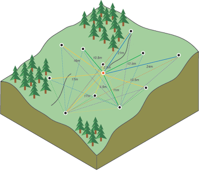
Often, each pair of locations has a unique distance, and there are often many pairs of points. To plot all pairs quickly becomes unmanageable. Instead of plotting each pair, the pairs are grouped into lag bins. For example, compute the average semivariance for all pairs of points that are greater than 40 meters apart but less than 50 meters. The empirical semivariogram is a graph of the averaged semivariogram values on the y-axis and the distance (or lag) on the x-axis (see diagram below).
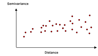
Spatial autocorrelation quantifies a basic principle of geography: things that are closer are more alike than things farther apart. Thus, pairs of locations that are closer (far left on the x-axis of the semivariogram cloud) should have more similar values (low on the y-axis of the semivariogram cloud). As pairs of locations become farther apart (moving to the right on the x-axis of the semivariogram cloud), they should become more dissimilar and have a higher squared difference (moving up on the y-axis of the semivariogram cloud).
Fitting a model to the empirical semivariogram
The next step is to fit a model to the points forming the empirical semivariogram. Semivariogram modeling is a key step between spatial description and spatial prediction. The main application of kriging is the prediction of attribute values at unsampled locations. The empirical semivariogram provides information on the spatial autocorrelation of datasets. However, it does not provide information for all possible directions and distances. For this reason, and to ensure that kriging predictions have positive kriging variances, it is necessary to fit a model—that is, a continuous function or curve—to the empirical semivariogram. Abstractly, this is similar to regression analysis, in which a continuous line or curve is fitted to the data points.
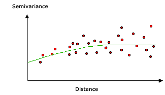
To fit a model to the empirical semivariogram, select a function that serves as your model—for example, a spherical type that rises and levels off for larger distances beyond a certain range (see the spherical model example below). There are deviations of the points on the empirical semivariogram from the model; some points are above the model curve, and some points are below. However, if you add the distance each point is above the line and add the distance each point is below the line, the two values should be similar. There are many semivariogram models from which to choose.
Semivariogram models
The Kriging tool provides the following functions from which to choose for modeling the empirical semivariogram:
- Circular
- Spherical
- Exponential
- Gaussian
- Linear
The selected model influences the prediction of the unknown values, particularly when the shape of the curve near the origin differs significantly. The steeper the curve near the origin, the more influence the closest neighbors will have on the prediction. As a result, the output surface will be less smooth. Each model is designed to fit different types of phenomena more accurately.
The diagrams below show two common models and identify how the functions differ:
A spherical model example
This model shows a progressive decrease of spatial autocorrelation (equivalently, an increase of semivariance) until some distance, beyond which autocorrelation is zero. The spherical model is one of the most commonly used models.
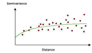
An exponential model example
This model is applied when spatial autocorrelation decreases exponentially with increasing distance. Here, the autocorrelation disappears completely only at an infinite distance. The exponential model is also a commonly used model. The choice of which model to use is based on the spatial autocorrelation of the data and on prior knowledge of the phenomenon.
More of the mathematical models are illustrated below.
Understanding a semivariogram—Range, sill, and nugget
As previously discussed, the semivariogram depicts the spatial autocorrelation of the measured sample points. Because of a basic principle of geography (things that are closer are more alike), measured points that are close will generally have a smaller difference squared than those farther apart. Once each pair of locations is plotted after being binned, a model is fit through them. Range, sill, and nugget are commonly used to describe these models.
Range and sill
When you look at the model of a semivariogram, you will notice that at a certain distance the model levels out. The distance where the model first flattens is known as the range. Sample locations separated by distances closer than the range are spatially autocorrelated, whereas locations farther apart than the range are not.
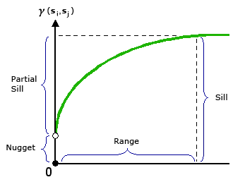
The value at which the semivariogram model attains the range (the value on the y-axis) is called the sill. A partial sill is the sill minus the nugget. The nugget is described in the following section.
Nugget
Theoretically, at zero separation distance (for example, lag = 0), the semivariogram value is 0. However, at an infinitely small separation distance, the semivariogram often exhibits a nugget effect, which is a value greater than 0. If the semivariogram model intercepts the y-axis at 2, then the nugget is 2.
The nugget effect can be attributed to measurement errors or spatial sources of variation at distances smaller than the sampling interval (or both). Measurement error occurs because of the error inherent in measuring devices. Natural phenomena can vary spatially over a range of scales. Variation at microscales smaller than the sampling distances will appear as part of the nugget effect. Before collecting data, it is important to gain an understanding of the scales of spatial variation in which you are interested.
Making a prediction
After you have uncovered the dependence or autocorrelation in your data (see Variography section above) and have finished with the first use of the data—using the spatial information in the data to compute distances and model the spatial autocorrelation—you can make a prediction using the fitted model. Thereafter, the empirical semivariogram is set aside.
You can now use the data to make predictions. Like IDW interpolation, kriging forms weights from surrounding measured values to predict unmeasured locations. As with IDW interpolation, the measured values closest to the unmeasured locations have the most influence. However, the kriging weights for the surrounding measured points are more sophisticated than those of IDW. IDW uses a simple algorithm based on distance, but kriging weights come from a semivariogram that was developed by looking at the spatial nature of the data. To create a continuous surface of the phenomenon, predictions are made for each location, or cell centers, in the study area based on the semivariogram and the spatial arrangement of measured values that are nearby.
Kriging methods
There are two kriging methods: ordinary and universal.
Ordinary kriging is the most general and widely used of the kriging methods and is the default. It assumes the constant mean is unknown. This is a reasonable assumption unless there is a scientific reason to reject it.
Universal kriging assumes that there is an overriding trend in the data—for example, a prevailing wind—and it can be modeled by a deterministic function, a polynomial. This polynomial is subtracted from the original measured points, and the autocorrelation is modeled from the random errors. Once the model is fit to the random errors and before making a prediction, the polynomial is added back to the predictions to give meaningful results. Universal kriging should only be used when you know there is a trend in your data and you can give a scientific justification to describe it.
Semivariogram graphs
Kriging is a complex procedure that requires greater knowledge about spatial statistics than can be conveyed in this topic. Before using kriging, you should have a thorough understanding of its fundamentals and assess the appropriateness of your data for modeling with this technique. If you do not have a good understanding of this procedure, it is strongly recommended that you review some of the references listed at the end of this topic.
Kriging is based on the regionalized variable theory that assumes that the spatial variation in the phenomenon represented by the z-values is statistically homogeneous throughout the surface (for example, the same pattern of variation can be observed at all locations on the surface). This hypothesis of spatial homogeneity is fundamental to the regionalized variable theory.
Mathematical models
Below are the general shapes and the equations of the mathematical models used to describe the semivariance.


References
Burrough, P. A. Principles of Geographical Information Systems for Land Resources Assessment. New York: Oxford University Press. 1986.
Heine, G. W. "A Controlled Study of Some Two-Dimensional Interpolation Methods." COGS Computer Contributions 3 (no. 2): 60–72. 1986.
McBratney, A. B., and R. Webster. "Choosing Functions for Semi-variograms of Soil Properties and Fitting Them to Sampling Estimates." Journal of Soil Science 37: 617–639. 1986.
Oliver, M. A. "Kriging: A Method of Interpolation for Geographical Information Systems." International Journal of Geographic Information Systems 4: 313–332. 1990.
Press, W. H., S. A. Teukolsky, W. T. Vetterling, and B. P. Flannery. Numerical Recipes in C: The Art of Scientific Computing. New York: Cambridge University Press. 1988.
Royle, A. G., F. L. Clausen, and P. Frederiksen. "Practical Universal Kriging and Automatic Contouring." Geoprocessing 1: 377–394. 1981.