You can apply the general steps you learned in The general suitability modeling workflow to implement your own suitability model using the Suitability Modeler.
You do not need to follow the steps sequentially in the Suitability Modeler. Instead, they are accomplished through a back-and-forth, iterative decision-making process. In the Suitability Modeler, you will gain insight into the model by interacting with the panes, plots, and maps. You can use these to define the transformation methods, weights, and spatial requirements for locating the sites.
The four general steps for creating a suitability model are as follows:
- Determine and prepare the criteria data.
- Transform the values of each criterion to a common suitability scale.
- Weight criteria relative to one another and combine them to create a suitability map.
- Locate the areas for the siting or to preserve.
Access the Suitability Modeler
You can access the Suitability Modeler by doing any of the following:
- In ArcGIS Pro, click the Suitability Modeler button
 on the Analysis tab.
 - In Catalog, open an existing suitability model.
- In Catalog, click a suitability model container
 , click New, and click Suitability Model.
When the Suitability Modeler pane appears, the following occur:
- The Suitability Modeler ribbon appears.
- A suitability model group layer is created in the Contents pane. This layer will store the model inputs and outputs.
- The Suitability Modeler pane appears, containing the Settings, Suitability, Locate, and Sources tabs. Settings is the active tab.
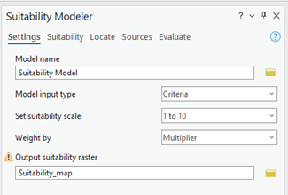
On the Settings tab, you can name the model, select the suitability scale, and indicate the method to use for weighting the criteria. Once you name the model and specify the model settings, click the Suitability tab to create the suitability map.
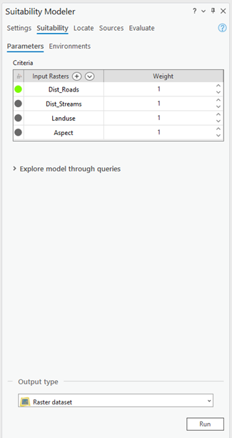
The Suitability tab and the accompanying Transformation pane are where you address the first three steps of the suitability workflow. Step 4, addressed on the Locate tab, is where you define the site or preservation area.
Step 1: Determine and prepare the criteria data
Some base data can be used directly as input criteria for the model. Other criteria must be derived using various Spatial Analyst geoprocessing tools. For example, the slope criterion is derived from the elevation raster using the Slope tool. You cannot derive data within the Suitability Modeler. However, you can switch back and forth between the Suitability Modeler and the geoprocessing tools.
To add criteria to the suitability model, do one of the following:
- Click the Add Criteria button
 on the Suitability ribbon.
 - Click the Add raster criteria dataset by browsing button
 in the Suitability pane.
 - Click the Add raster criteria as layers from contents button
 in the Suitability pane.
 - Drag a layer from the Contents pane into the suitability group layer.
- Right-click the suitability group layer and click Add Data
 .
.
As each criterion is added to the Criteria table, it is also added to the suitability group layer in the Contents pane.
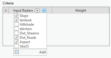
Step 2: Transform the values of each criterion to a common suitability scale
To transform a criterion to a common suitability scale, click the circle button next to the criterion in the criteria list on the Suitability tab. The following occur:
- The Transformation Pane appears.
- A transformed layer of the criterion is added to the suitability group layer in the Contents pane.
- A default transformation is applied based on the type of the input values.
The button next to the criterion turns green, indicating it is the active criterion in the Transformation Pane. The button turns grey once the criterion has been transformed and is no longer the active criterion in the Transformation pane.
The three transformation methods that can be applied to the criterion values are Unique Categories, Range of Classes, and Continuous Functions.
Unique Categories
The Unique Categories method is best for categorical data such as land use types. This method is a one-to-one matching of the criterion value to the suitability value.
Range of Classes
The Range of Classes method is best for continuous data, in which ranges of values can be grouped into homogeneous classes that can be assigned the same suitability preference.
Continuous Functions
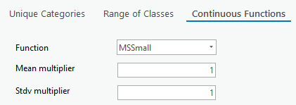
The Continuous Functions method is best for criteria represented by continuous values such as slope, aspect, or distance from streams. This method applies linear and nonlinear functions to transform the values continuously to the suitability scale. Because this method applies a continuous function to the criterion values, with each increase in the criterion value, the resulting suitability value continuously changes. For example, the suitability may exponentially decrease with each step away from a stream.
The Continuous Functions method is the most commonly used transformation method for continuous data.
Default transformation methods
The default transformation methods for a criterion depend on the type and number of unique values in the raster. The following table lists those conditions:
| Criterion condition | Transformation method |
|---|---|
The criterion has < 27 integer values. | Unique Categories |
The criterion has >= 27 integer values. | Range of Classes |
The criterion has floating-point values. | Continuous Functions |
You can apply a transformation method other than the default. As you click each method or function in the Continuous Functions method, parameters applicable to the method or function appear, allowing you to further refine the transformation.
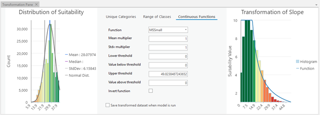
The Transformation pane has three sections you can use to select the best transformation method for the input criteria values.
A histogram of the final suitability values is on the left.
You can use the plot on the right to help you select transformation methods and functions. The plot depicts how the input values will be converted to the suitability scale. In the plot, the x-axis contains the base criterion input values, the y-axis contains the suitability scale, and a histogram of the base criterion values is displayed. For the Continuous Functions method, the function being applied is overlaid on the plot. As different methods or functions are applied, the plot is updated.
As you explore the methods and functions and their parameters, the transformation plot, the final suitability histogram, and the transformed and final suitability map layers in the suitability group layer in the Contents pane are updated. This updating provides feedback about the effects that transformation will have on the transformed criterion as well as the impact to the final suitability map.
Once you determine the best transformation to capture the preference for the values within the criterion, you transform the next criterion, and repeat the process until all criteria are transformed.
Step 3: Weight criteria relative to one another and combine them to create a suitability map
Now you weight the criteria relative to one another. There are two methods that can be used to weight the criteria, multiplier or percent. If you specified the Multiplier method for the Weight by parameter on the Settings tab, the transformed criterion values are multiplied by this value. The multiplied transformed criterion values are then added together. A weight of 2 means the criterion is twice as important as a criterion with a weight of 1. A weight of 10 means the criterion is 10 times more important. Common weights are between 1 and 2. This method is best when you can directly weight the criteria relative to one another. Use the spinner controls to adjust the weight for each criterion.
If you specified the Percent method in the Weight by parameter on the Settings tab, once the percentages are applied and the criteria are added, the range of the output values in the resulting suitability map are linearly transformed to the suitability scale set on the Settings tab. By default, that range is 1 to 10. The sum of the criteria's percent must equal 100 percent. This method is best when you want to indicate how much each criterion influences the resulting suitability map. Use the Weight sliders to adjust the percentage.
As the weights are altered, the histogram of the final suitability map in the Transformation pane and the final suitability map in the suitability group layer in the Contents pane are updated. A suitability map at screen resolution has been created, identifying the relative preference of each location based on the attributes at the location.
You can explore the input criteria, the applied transformations, the specified weights, and their effects on the final suitability layer using queries in the Explore model through queries drop down on the Suitability tab. Once you are satisfied with the specifications for the final suitability layer, you'll locate the areas for siting or preservation.
Step 4: Locate the areas for the siting or to preserve
On the Locate tab, specify the spatial requirements for the suitability model. Up to this point, the calculations were performed only on the data presented at the display extent and resolution. Before you locate your areas, run the model at the full resolution and extent of the source input. To do this, click the Run button on the Suitability tab.
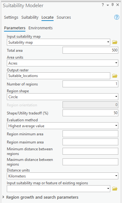
The resulting suitability map is the input to the Locate tab. The locate component of the suitability modeling process allows the spatial requirements to be specified. The total area, number of regions, and shape characteristics of the desired areas are identified. You can also specify the minimum and maximum region sizes and distances between regions. Click Run on the Locate tab or the Run button  on the Suitability ribbon. A new Locate layer that identifies the best locations to site or preserve is added to the suitability group layer in the Contents pane.