Interpreting Exploratory Regression results—ArcGIS AllSource

When you run the Exploratory Regression tool, the primary output is a report. The report is written as geoprocessing messages while the tool runs and can also be accessed from the project geoprocessing history. You can also output a table to help you further investigate the models that have been tested. One purpose of the report is to help you determine whether the candidate explanatory variables yield any properly specified OLS models. In the event that no models meet all of the criteria you specified when you launched the Exploratory Regression tool, the output will still reveal which variables are consistent predictors and help you determine which diagnostics are giving you problems. Strategies for addressing problems associated with each of the diagnostics are provided in What they don't tell you about regression analysis and Regression analysis basics (see Common regression problems, consequences, and solutions). For more information about how to determine whether you have a properly specified OLS model, see Regression analysis basics.

Report details

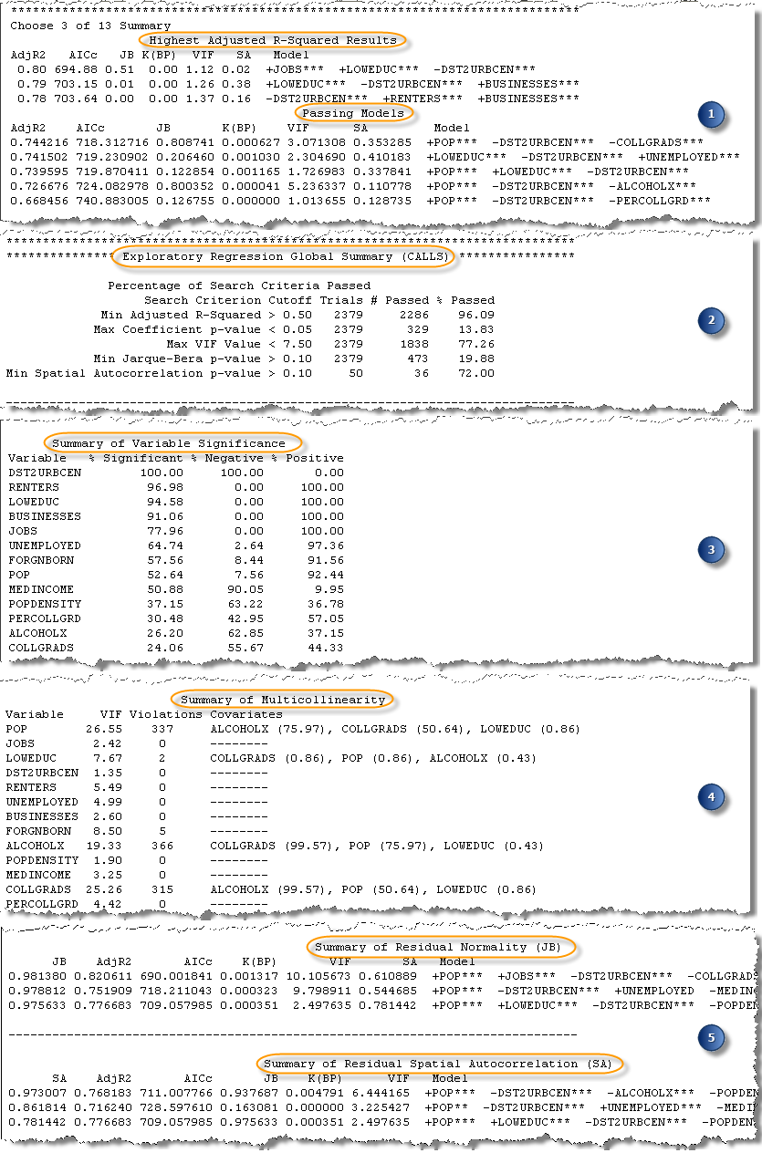
The Exploratory Regression tool report has five sections. Each section is described below.

Best models by number of explanatory variables

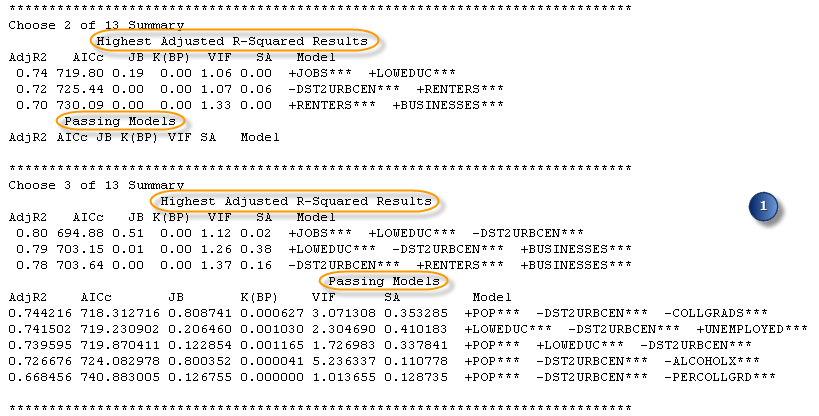
The first set of summaries in the output report is grouped by the number of explanatory variables in the tested models. If you specify 1 for the Minimum Number of Explanatory Variables parameter, and 5 for the Maximum Number of Explanatory Variables parameter, you will have five summary sections. Each section lists the three models with the highest adjusted R² values and all of the passing models. Each summary section also includes the diagnostic values for each listed model: corrected Akaike Information Criteria—AICc, Jarque-Bera p-value—JB, Koenker’s studentized Breusch-Pagan p-value—K(BP), the largest Variance Inflation Factor—VIF, and a measure of residual Spatial Autocorrelation (the Global Moran’s I p-value)—SA. These summaries give you an estimate of how well your models are predicting (Adj R²), and whether any models pass all of the diagnostic criteria you specified. If you accepted all of the default search criteria (Minimum Acceptable Adj R Squared, Maximum Coefficient p-value Cutoff, Maximum VIF Value Cutoff, Minimum Acceptable Jarque Bera p-value, and Minimum Acceptable Spatial Autocorrelation p-value parameters), any models included in the Passing Models list will be properly specified OLS models.

If there aren’t any passing models, the rest of the output report still provides useful information about variable relationships and can help you make decisions about how to move forward.

Exploratory Regression Global Summary

The Exploratory Regression Global Summary section is an important place to start, especially if you haven't found any passing models, because it shows you why none of the models are passing. This section lists the five diagnostic tests and the percentage of models that passed each of those tests. If you don’t have any passing models, this summary can help you determine which diagnostic test is causing issues.

Often the diagnostic that is causing problems is the Global Moran’s I test for Spatial Autocorrelation (SA). When all of the tested models have spatially autocorrelated regression residuals, it most often indicates that you are missing key explanatory variables. One of the best ways to find missing explanatory variables is to examine the map of the residuals that are output by the Ordinary Least Squares regression (OLS) tool. Choose one of the exploratory regression models that performed well for all of the other criteria (use the lists of highest adjusted R-squared values, or select a model from those in the optional output table), and run OLS regression using that model. Output from the Ordinary Least Squares regression (OLS) tool is a map of the model residuals. You should examine the residuals to see whether they provide any clues about what may be missing. Try to think of as many candidate spatial variables as you can (for example, distance to major highways, hospitals, or other key geographic features). Consider trying spatial regime variables: if all of your underpredictions are in the rural areas, for example, create a placeholder variable to see whether it improves your exploratory regression results.

The other diagnostic that is commonly problematic is the Jarque-Bera test for normally distributed residuals. When none of your models pass the Jarque-Bera (JB) test, there is a problem with model bias. Common sources of model bias include the following:

Nonlinear relationships
Data outliers

Viewing a scatterplot matrix of the candidate explanatory variables in relation to your dependent variable will show you whether you have either of these problems. Additional strategies are outlined in Regression analysis basics. If your models are failing the SA test, fix those issues first. The bias may be the result of missing key explanatory variables.

Summary of Variable Significance

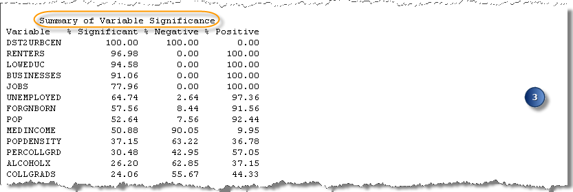
The Summary of Variable Significance section provides information about variable relationships and how consistent those relationships are. Each candidate explanatory variable is listed with the percentage of times it was statistically significant. The first few variables in the list have the largest values for the % Significant column. You can also see how stable variable relationships are by examining the % Negative and % Positive columns. Strong predictors will be consistently significant (% Significant), and the relationship will be stable (primarily negative or primarily positive).

This part of the report can also help you be more efficient. This is especially important when you are working with a large number of candidate explanatory variables (more than 50) and want to try models with five or more predictors. When you have a large number of explanatory variables and are testing many combinations, the calculations can take a long time. In some cases, the tool won’t finish at all due to memory errors. A best practice is to gradually increase the number of models tested: start by setting both the Minimum Number of Explanatory Variables and Maximum Number of Explanatory Variables parameters to 2, then to 3, then to 4, and so on. With each run, remove the variables that are rarely statistically significant in the tested models. This Summary of Variable Significance section will help you find those variables that are consistently strong predictors. Even removing one candidate explanatory variable from your list can significantly reduce the time it takes for the Exploratory Regression tool to complete.

Summary of Multicollinearity

You can use the Summary of Multicollinearity section of the report in conjunction with the Summary of Variable Significance section to understand which candidate explanatory variables can be removed from your analysis to improve performance. The Summary of Multicollinearity section tells you how many times each explanatory variable was included in a model with high multicollinearity, and the other explanatory variables that were also included in those models. When two (or more) explanatory variables are frequently found together in models with high multicollinearity, it indicates that those variables may be providing the same results. Since you only want to include variables that explain a unique aspect of the dependent variable, consider choosing only one of the redundant variables to include in further analysis. One approach is to use the strongest of the redundant variables based on the Summary of Variable Significance results.

Additional diagnostic summaries

The final diagnostic summaries show the highest Jarque-Bera p-values (Summary of Residual Normality) and the highest Global Moran’s I p-values (Summary of Residual Autocorrelation). To pass these diagnostic tests, you are looking for large p-values.

These summaries are not especially useful when your models are passing the Jarque-Bera and Spatial Autocorrelation (Global Moran’s I) test, because if your criteria for statistical significance is 0.1, all models with values larger than 0.1 are equally passing models. These summaries are useful, however, when you do not have any passing models and you want to see how far you are from having normally distributed residuals or residuals that are free from statistically significant spatial autocorrelation. For instance, if all of the p-values for the Jarque-Bera summary are 0.000000, it's clear that you are far away from having normally distributed residuals. Alternatively, if the p-values are 0.092, you're close to having residuals that are normally distributed (in fact, depending on the level of significance that you chose, a p-value of 0.092 may be passing). These summaries demonstrate how serious the problem is and, when none of your models are passing, they indicate which variables are associated with the models that are getting close to passing.

Table details

If you provided a value for the Output Results Table parameter, a table will be created containing all models that met your Maximum Coefficient p-value Cutoff and Maximum VIF Value Cutoff criteria. Even if you do not have any passing models, it is likely that you will have some models in the output table. Each row in the table represents a model meeting your criteria for coefficient and VIF values. The columns in the table provide the model diagnostics and explanatory variables. The listed diagnostics are Adjusted R-Squared (R2), corrected Akaike Information Criteria (AICc), Jarque-Bera p-value (JB), Koenker’s studentized Breusch-Pagan p-value (BP), Variance Inflation Factor (VIF), and Global Moran’s I p-value (SA). You may want to sort the models by their AICc values. The lower the AICc value, the better the model performed. You can sort the AICc values in ArcMap by double-clicking the AICc column. If you are choosing a model to use in an OLS analysis (to examine the residuals), be sure to choose a model with a low AICc value and passing values for as many of the other diagnostics as possible. For example, if you have looked at your output report and you know that Jarque-Bera was the diagnostic that caused issues, look for the model with the lowest AICc value that met all of the criteria except for Jarque-Bera.

Additional resources

If you’re new to regression analysis in ArcGIS, it is recommended that you watch Regression Analysis: Building a Regression Model Using ArcGIS Pro then complete the Regression Analysis tutorial.

You can also see the following resources:

Learn more about how Exploratory Regression works
What they don't tell you about regression analysis
Regression analysis basics
Burnham, K.P., and D.R. Anderson. 2002. Model Selection and Multimodel Inference: A Practical Information-Theoretic Approach, 2nd Edition. New York: Springer. Section 1.5.

Feedback on this topic?