You can evaluate the quality and distribution of values in each field in your data using data engineering. For example, the number of null values in a field may be a helpful data quality metric when identifying features with missing data. Descriptive statistics, such as the mean, standard deviation, and kurtosis, may help you understand the distribution of values in the fields as well as assess how to proceed when using a field in an analysis.
The Data Engineering view in ArcGIS AllSource allows you to display descriptive statistics and metrics for fields of interest in your data in a table format. Each field is displayed as a row and each statistic as a column. You can use this table to explore the data or correct issues in the data by setting symbology, creating charts, and running geoprocessing tools that are relevant to each metric and property for the selected field.
Select fields and calculate statistics
When you open the Data Engineering view, it contains two panels: one displays the fields in your data, and the other displays a statistics table for the fields (once they have been selected and calculated).
Learn more about the Data Engineering view
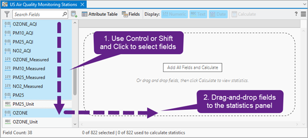
To get started, click a single field in the fields panel, press Ctrl and click to select individual, separate fields, or press Shift and click to select multiple fields. Then drag the fields to the statistics panel.

Alternatively, right-click selected fields and click Add To Statistics or Add To Statistics And Calculate.
Note:
You can also add and calculate all fields in one action by clicking the Add Fields and Calculate Statistics button  on the toolbar of the Fields Panel or by clicking the Add All Fields and Calculate button in the middle of the empty statistics panel prior to adding fields.
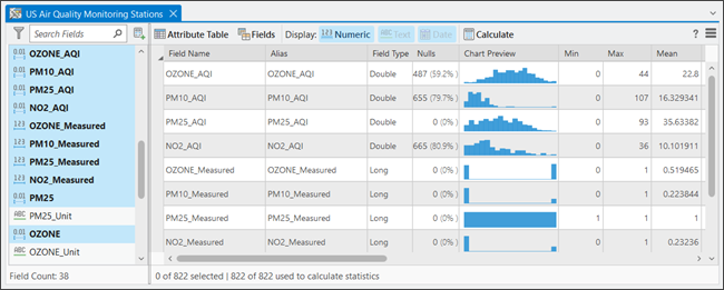
Once the fields are added, they are displayed as rows in the statistics table. Each row contains the field name, alias, and data type of the selected fields. Additionally, a series of statistics columns appear that will contain additional information about the selected fields once calculations are made.
To populate the statistics columns for the selected fields, click the Calculate button. While the statistics are being calculated, the Calculate button changes to a Cancel button that you can click to cancel the calculation.

The statistics columns are populated with information for each field of the data.

If you have selected records, the results correspond to the selected records in the data. The number of selected features and the number of features that were used to calculate statistics are shown below the statistics table.
If you have pending edits in the feature layer or table, the pending edits are used in the calculation.
Types of statistics
In the Data Engineering view, you can calculate and display statistical and data quality metrics of each field in the data as columns in a table. In the table, some of the header names of the statistics are abbreviated. Hover over the header to view the entire name of the statistic. The results in the statistics table are displayed to 6 decimal places. You can right-click a cell and choose the Copy option to copy the raw value.
Note:
For fields with data type timestamp offset or time only, consider the following:
- Statistics for fields with data type timestamp offset are calculated and displayed in UTC (offset +00:00:00).
- Statistics for fields with data type time only are linear statistics, not circular statistics.
Once values are calculated, right-click the statistics cells for each field to access additional functionality related to the statistics. Some of this functionality uses geoprocessing tools that modify the input data. If the data is not editable, make an editable copy of it before you begin data engineering.
| Statistic | Description | Applicable data types | Menu options |
|---|---|---|---|
Nulls | A count and percent of the total number of records containing null values in the field. To select records containing null values, right-click cells in this column. Note:If the symbology of the layer is not configured to display null values, the selection may not appear on the map. Configure symbology to show values out of range to display features with nulls. | Numeric, Text, Date |
|
Chart Preview | A visual representation of the distribution of values in the field. Histograms are displayed for numeric fields (short, long, big integer, float, double), bar charts for categorical fields (text), and line charts for date fields (date, date only, time only, timestamp offset). Use the chart preview column to perform an initial exploration. To create charts for fields of interest, right-click cells in this column. Note:Histograms and line charts are displayed with 20 bins by default. Depending on the sparsity of the data, there may be bins that contain no data, and bins with empty values are treated as zero in the chart preview. To change the level of detail, right-click the chart preview and create a chart. You can hover over bar charts and line charts to display a ToolTip with additional information. For bar charts, the ToolTip displays the most frequent categories, and for line charts, the ToolTip describes the amount and duration of intervals in the chart. Note:For interval descriptions of date fields, months are considered to be 30 days. For example, an interval of 3.2 months corresponds to 96 days. | Numeric, Text, Date |
|
Minimum (Min) | The smallest value in the field. To select records containing the minimum value, right-click cells in this column. | Numeric, Date |
|
Maximum (Max) | The largest value in the field. To select records containing the maximum value, right-click cells in this column. | Numeric, Date |
|
Mean | The mean of all values in the field. The mean is the average value in a distribution, calculated as the sum of the values divided by the total count of values in the field. The mean is the most common measure of central tendency in a distribution. To calculate the mean date for date fields, each date is converted to a number by calculating the difference between the date and a reference date (for example, 1900-01-01), calculated in milliseconds. The sum of all millisecond values divided by the count of date values provides the mean date, which is rounded to the nearest second for display purposes. For fields with data type date only, the time is assumed to be midnight for calculation purposes. Note:The mean date may not be in the same temporal resolution (i.e., minutes, seconds, milliseconds) as the values in the field. To select records containing values above and below the mean, right-click cells in this column. | Numeric, Date |
|
Standard Deviation (Std. Dev.) | The standard deviation for values in the field. The standard deviation is a measure of the spread of the distribution. It is calculated as the square root of variance, in which the variance is the average of the squared difference of each value from the mean of the field. | Numeric |
|
Median | The median for all values in the field. The median is the middle value in the sorted list of values. If there is an even number of values, the median is the mean between the two middle values in the distribution. To select records containing values above the median and values below the median, right-click cells in this column. | Numeric, Date |
|
Count | The count and percent of the total number of nonnull values in the field. | Numeric, Text, Date |
|
Number of Unique Values (Unique) | The number of unique values in the field. | Numeric, Text, Date | No unique actions |
Mode | The mode for all values in the field. The mode is the most frequently occurring value in the field. In the case of ties, when the most frequently occurring value in a field corresponds to multiple values, the cell displays [Multiple Values], and you can hover over the cell to display the mode values and their frequency. When all values in the field are unique, the cell displays [All Unique Values]. To select records containing the mode, right-click cells in this column. | Numeric, Text, Date |
|
Least Common | The least common value in the field. In the case of ties, when the least common value in a field corresponds to multiple values, the cell displays [Multiple Values], and you can hover over the cell to display the least common values and their frequency. When all values in the field are unique, the cell displays [All Unique Values]. To select records containing the least common value, right-click cells in this column. | Numeric, Text, Date |
|
Outliers | The number of records with outlier values in the field. Outliers are values that are more than 1.5 times the interquartile range above the third quartile or below the first quartile of the selected field. To select records containing the outlier values (or all values except outliers), right-click cells in this column. | Numeric |
|
Sum | The sum of all values in the field. | Numeric | No unique actions |
Range | The difference between the smallest and largest values in the field. For date fields, the range provides the time span between the earliest date and latest date found in the field. Note:For date field ranges, months are considered to be 30 days. For example, a range of 3.2 months corresponds to 96 days. | Numeric, Date | No unique actions |
Interquartile Range (IQR) | The range between the first quartile and the third quartile values in the field. Quartiles divide the sorted list of values into four groups containing equal numbers of values. The first quartile value is the upper limit of the first group in ascending order, and the third quartile is the upper limit of the third group. To select records containing values within this range, right-click cells in this column. | Numeric |
|
First Quartile (Q1) | The value of the first quartile in the field. Quartiles divide the sorted list of values into four groups containing equal numbers of values. The first quartile value is the upper limit of the first group in ascending order. In the case of ties, the mean of all corresponding values is shown. To select records containing values above and below the first quartile, right-click cells in this column. | Numeric, Date |
|
Third Quartile (Q3) | The value of the third quartile in the field. Quartiles divide the sorted list of values into four groups containing equal numbers of values. The third quartile is the upper limit of the third group. In the case of ties, the mean of all corresponding values is shown. To select records containing values above and below the third quartile, right-click cells in this column. | Numeric, Date |
|
Coefficient of Variation (CV) | The coefficient of variation for values in the field. The coefficient of variation is a measure of the relative spread of the values. It is calculated as the standard deviation divided by the mean of the field. Unlike the standard deviation, which must always be considered in the context of the range of the data, the coefficient of variation provides a way to compare data series with different ranges and means. The coefficient of variation cannot be calculated if the mean value is equal to zero. If the mean value is close to zero and there are both positive and negative values in the dataset, the coefficient of variation may lack meaningful interpretation. | Numeric | |
Skewness | The skewness of values in the field. Skewness measures the symmetry of the distribution. Skewness is zero (or close to zero) if the distribution is symmetrical on both sides, as seen in a normal distribution. Distributions with longer tails on the left have negative skewness, and distributions with longer tails on the right have positive skewness. The skewness is calculated as the third moment (the average of the cubed data values) divided by the cubed standard deviation. | Numeric | |
Kurtosis | The kurtosis of values in the field. Kurtosis describes the heaviness of the tails of a distribution compared to the tails of a normal distribution, helping identify the frequency of extreme values. Distributions with kurtosis less than three have lighter tails and fewer extreme values than the normal distribution, and distributions with kurtosis greater than three have heavier tails and more extreme values than the normal distribution. The kurtosis is calculated as the fourth moment (the expected value of the data values taken to the fourth power) divided by the fourth power of the standard deviation. | Numeric |
Interactive statistics table
The statistics table is interactive. Right-click cells and headers and use the toolbar to access functionality.
Interact with fields
Right-click a row header to access functionality applicable to the selected field such as the following:
- Create Chart—Create charts using the selected field. Recommendations are provided based on the data type.
- Fields—Open the fields view and set the current field as the active field in the view.
- Attribute Table—Open the attribute table and set the current field as the active field in the attribute table.
- Clean, Construct, Integrate, and Format—Access geoprocessing tools to prepare the data. See Prepare data to learn more about these options.
- Remove Field—Remove the field and clear its statistics from the statistics table.
Note:
Most geoprocessing operations that modify the input data cannot be undone.

Interact with cells
Right-click a cell to access functionality applicable to the selected cell. All cells allow Copy to copy the cell's value to the clipboard. For cells in the Chart Preview column, you can open the default chart of the cell or create a chart applicable to the data type of the cell. For all other columns, context-sensitive selection and geoprocessing tool options are available. For example, the Standard Deviation column allows selection of records within one, two, or three standard deviations of the mean value and contains links to the Standardize Field and Transform Field tools. For a list of all applicable options and functions for each column, see the table in the Types of statistics section above.
Note:
Context-sensitive selection is disabled in the following two cases:
- When the calculated statistics were performed on a selection. To make selections on calculated statistics from a selection on a layer, you can create a selection layer.
- When the field of a selected cell has data type float or double.
Display specific data types
The statistics table toolbar includes options to designate which fields and statistics columns are displayed based on data type.

For example, you can click the Text option to remove fields of data type text. The Numeric button will hide and display fields with data type short, long, big integer, float, and double. The Date button will hide and display fields with data type date, date only, time only, and timestamp offset.
When you remove data types from the statistics table, the columns that are unique to the removed data type are also removed. This can make it easier to review the table for items of interest. For example, if you display only fields of type date, columns that describe distributions, such as skewness and kurtosis, are omitted, so the number of columns is reduced to only those of interest.
Sort, hide, freeze, and reorder columns
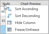
By default, the fields display in the same order that they appear in the attribute table. The options for the column headers allow you to sort, hide, and freeze the columns in the table.

Sorting allows you to reorder the rows by the value in the calculated statistic. For example, you can sort fields by the Nulls column to learn which fields may have missing data.
Note:
You can only sort if the table contains fields with a single data type. Use the display options on the toolbar to filter to a specific data type; then sort. The sort order is reset to the default each time a new field is added to the statistics table.
Click Freeze/Unfreeze to move the column to the beginning of the statistics table and lock it in place so that the column displays as you scroll the table horizontally. To reorder the columns, drag a column header to the new location.
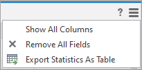
To hide columns, click Hide Column. This removes the column from view. To show all hidden columns, click Show All Columns.

To remove all the fields and their statistics from the statistics table, click Remove All Fields. If a removed field is added back to the statistics table, you will need to click the Calculate button again to view its statistics.
Export statistics
To use the statistics in other parts of ArcGIS AllSource, persist the statistics as a stand-alone table. Click Export Statistics As Table to open the Field Statistics To Table tool. This option allows you to export the statistics as a single table or as separate tables for each data type. This tool does not support statistics for fields of data type big integer, date only, time only, and timestamp offset.
References
- Sheskin, D.J. (2000). "Handbook of Parametric and Nonparametric Statistical Procedures." Second Edition. Boca Raton, Florida: Chapman & Hall/CRC. ISBN: 978-1-58488-814-7.
- UCLA: Statistical Consulting Group.
"IEEE Standard for Floating-Point Arithmetic." IEEE Std 754-2019 (Revision of IEEE 754-2008), vol., no., pp.1-84, 22 July 2019. https://ieeexplore.ieee.org/document/8766229.