Available with Network Analyst license.
The ArcGIS Network Analyst extension allows you to use historical traffic information to model the time-dependent speeds of traveling on roads. This way, your expected travel and arrival times are more reliable, and the time you actually spend driving is likely to be less than if traffic patterns were ignored.
Tip:
The Network Analyst tutorial data, which is available on ArcGIS.com, includes a San Francisco geodatabase with traffic data. Studying the Streets feature class, the DailyProfiles table, and the Streets_DailyProfiles table contained in the SanFrancisco.gdb file will complement what you learn in this topic. After downloading and extracting the data, you can find the SanFrancisco geodatabase at \Network Analyst\Tutorial\SanFrancisco.gdb.
Note:
Traffic can only be configured in a geodatabase; it cannot be configured in a shapefile-based network dataset.
Historical traffic attribute properties
The Historical Traffic tab displays the properties that can be configured on a network dataset that supports historical traffic.
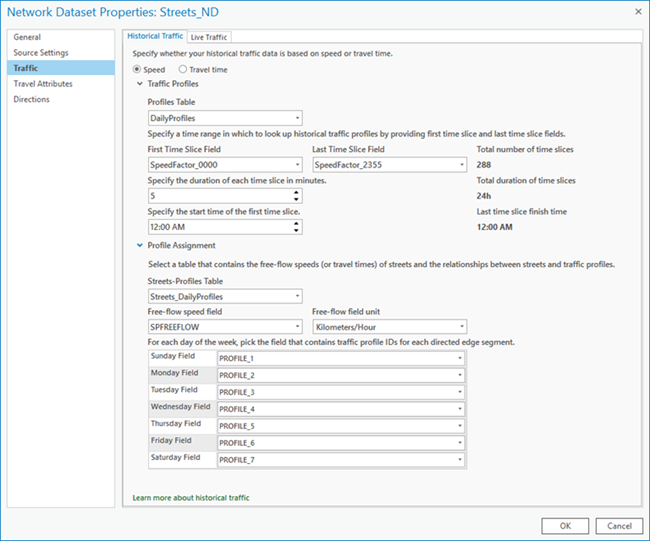
- Speed—Choose Speed if historical traffic data is speed based.
- Travel time—Choose Travel time if historical traffic data is time based.
- Traffic Profiles—Use the following table to set the properties for the Traffic Profiles table:
Property Description Profiles Table
The name of the table that contains traffic profiles.
First Time Slice Field
This property, in conjunction with Last Time Slice Field, specifies a time range in which to look up historical traffic profiles. Whenever an edge is evaluated for a time of day outside the range, its multiplier is assumed to be one. This assumption hastens the lookup of costs for times of the day when there is little to no traffic.
Last Time Slice Field
See the description for First Time Slice Field.
Specify the duration of each time slice in minutes
The traffic profiles table must be divided into equal time intervals throughout the day. This property specifies the length of the interval in minutes.
Specify the start time of the first time slice
This property identifies the time of day that the beginning of the First Time Slice Field represents.
For example, if the First Time Slice Field is set to SpeedFactor_0000, which starts at 12:00 a.m., the start time for the first time slice is set to 12 AM.
Last time slice finish time
This property specifies the time of day that the end of the Last Time Slice Field represents. It is automatically deduced from the number of time-slice fields and the duration of each time slice in minutes value.
- Profile Assignment—This section assigns profiles to street segments and establishes baseline values.
Property Description Streets-Profiles Table
The name of the table that contains the free-flow speeds (or travel times) of streets and the relationships between streets and traffic profiles.
Free-flow travel time field or Free-flow speed field
The name of this property changes depending on whether Travel Time or Speed is chosen for the historical traffic data. This property indicates the field that contains free-flow travel times, or free-flow travel speeds if the data is speed based.
Free-flow field unit
This property indicates the time units of the field specified in Free-flow travel time field, or the speed units in Free-flow speed field if the data is speed based.
- Sunday Field
- Monday Field
- Tuesday Field
- Wednesday Field
- Thursday Field
- Friday Field
- Sunday Field
- Saturday Field
The name of the field that contains traffic profile IDs for Sunday traffic, Monday traffic, and so on.
Create historical traffic data for use with Network Analyst
Even if you obtain your data from a third party, it's important to understand how historical traffic data is created so that you can properly configure it in a network dataset. This section describes the model that Network Analyst uses.
Because traffic data captures the continual ebb and flow of travel speeds, each travel direction of an edge can have many differing costs depending on the time of day. This is in contrast to a typical cost attribute, which allows only one value per edge direction.
There are several ways to model multiple costs per edge direction. To understand why Network Analyst uses a particular model, it is important to understand the typical way to model traffic.
Typical historical traffic model
One option for storing historical traffic data is to create a series of costs for each edge. The costs represent traffic speeds at different times of the day, over the course of a week. For example, a week can be partitioned into 168 discrete, one-hour intervals. This means that each edge needs 168 cost attributes to represent how traffic tends to change over a week's time. If the time span is shortened to 5-minute intervals to provide better temporal resolution, each edge needs 2,016 cost attributes. Storing all these unique values requires a lot of space, especially for large networks. Also, since many streets have the same costs during the day, there is a lot of unnecessary duplication of data. For these reasons, this modeling option isn't viable for Network Analyst.
Network Analyst historical traffic model
Rather than store all the traffic information on a per-feature basis, ArcGIS uses a normalized model to minimize the size of the traffic data. Instead of storing the 168 or 2,016 cost attributes per feature, a related table is created to hold this information. Each row in the table contains the speeds or, optionally, travel times for each interval in a day. A row is a traffic profile; it represents how speeds change throughout the day. For example, if you have many secondary, 35-mile-per-hour streets with travel speeds that vary in unison throughout the day, you can create a single row in the traffic profiles table to represent these dynamics and have these streets point to the same row, or traffic profile. Further refinements are made so that even roads with differing speed limits that follow the same traffic pattern throughout the day can refer to the same traffic profile.
To better understand this traffic model, assume you need to use it to record and store travel speeds for a one-way street segment over the course of a week, starting on Monday. First, you would determine the free-flow speed, which is the speed a vehicle travels when no other traffic is impeding its movement. The method you use to determine the free-flow speed is your choice, but it is typically the speed limit or the observed, average speed of cars that pass by when other vehicles aren't present. Say you choose the observed, average speed of cars and establish the free-flow speed is 70 miles per hour.
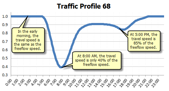
Now you can make observations throughout the day at equal time intervals, or time slices. The intervals you choose give your data its temporal resolution. You could choose 1-hour intervals, 10-minute intervals, and so on. Say you choose 5-minute intervals. Your observations are recorded as scale factors of the free-flow speeds. The scale factors are limited to a range of zero to one. Assume you observe cars traveling 28 miles per hour at 8:00 a.m. This is 0.4 times the free-flow travel speed. At 5:00 p.m., the average speed is 60 miles per hour, which is about 0.85 times the free-flow travel speed. At 11:00 p.m., there are few cars on the road, and their average speed is 70 miles per hour, which is equal to the free-flow travel speed—the scale factor is one.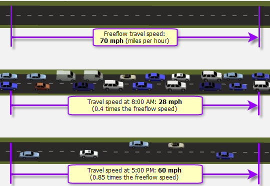
Once your observations for the day are completed, you need to reference a table of traffic profiles and choose the one profile that best matches the observed variation of relative speeds throughout the day.
You choose traffic profile 68 (plotted in the graph below) to represent the segment's travel time on Mondays.
Note:
The time of day in a profile always represents local time, that is, the time zone in which the referencing edge is located. Therefore, an edge in Los Angeles that references profile 68 will have a speed that is 40 percent of free-flow speed at 8:00 a.m. pacific standard time. An edge in New York that points to the same profile will have a speed that is 40 percent of the free-flow speed at 8:00 a.m. eastern standard time.
When you have a large number of profiles, you have the potential to more accurately model travel times. However, when you have fewer profiles, the space requirements for the data are reduced. The objective is to find a good balance between accuracy and space requirements. It is common for large street networks to have anywhere from dozens to hundreds of traffic profiles.
Now that you've chosen a profile for Mondays, you need to repeat the process for the other days of the week. The process is summarized below:
- Observe or calculate the free-flow travel speeds on the street segment. (This doesn't need to be repeated, since it's the same, regardless of the day of the week.)
- Observe average speeds for equal intervals throughout the day.
- Convert the speeds to a scale factor (between 0 and 1) of the free-flow speed. (If you're directly modeling travel times instead of speeds, the scale factor must be greater than or equal to one.)
- Choose a profile to represent the street segment's traffic for that day of the week.
You determine that traffic profile 68 also works well for the segment on all other weekdays. This determination is often made, since general traffic patterns are frequently the same on all business days. Still, it's not difficult to find weekdays that use different representative profiles; for example, it could be that Mondays, Tuesdays, and Wednesdays use the same profile, while Thursdays and Fridays share a different profile.
The Saturday and Sunday traffic on your segment is light and steady, so you choose Traffic Profile 3 (below) to represent travel times on the weekends.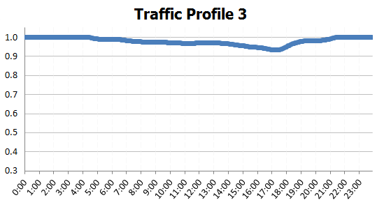
Next, you store the free-flow speeds and the relationships between the street segment and traffic profiles in a table: the Streets-Profiles table. The next sections review this table, as well as other required inputs.
Store data and relationships in the geodatabase
You need one or more line feature classes and two tables in a geodatabase to create a network dataset with historical traffic data. The line feature classes represent streets, which must be stored in a feature dataset. The speed profiles are stored in one of the tables, and the relationships between the streets and speed profiles are stored in the other table. These items and the fields required to set up historical traffic on a network dataset are described in the following subsections.
Note:
The relationships between streets and speed profiles are made by storing values of unique identifiers in tables; you don't need to create any relationship classes.
Streets feature class
Each street feature has a unique identifier: the ObjectID value. The Streets-Profiles table relates streets to their various traffic profiles through the unique identifier.
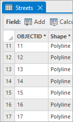
Other fields may be useful when setting up historical traffic. They are listed below and described in more detail later in this topic.
| Field | Field name examples | Description |
|---|---|---|
Time-independent travel times | FT_Minutes TF_Minutes | Create a network cost attribute that is used when sequencing locations in a route or vehicle routing problem analysis that uses traffic. |
Weekday travel times | FT_WeekdayMinutes TF_WeekdayMinutes | Create a network cost attribute that is used when a street segment doesn't have an associated historical traffic profile for a weekday. (The time-neutral travel times are often also used as weekday-specific travel times.) |
Weekend travel times | FT_WeekendMinutes TF_WeekendMinutes | Create a network cost attribute that is used when a street segment doesn't have an associated traffic profile for a Saturday or Sunday. |
Time zone | TimeZoneID | Create a time-zone network attribute that is needed when a network spans multiple time zones. |
Profiles table
Each record in a traffic profiles table has a unique identifier and several fields for storing the free-flow scale factor at different times of the day. The times of the day are split into time intervals, or time slices, which must be of equal duration and, thus, split a 24-hour period into equal intervals. For instance, if the time slices are 5 minutes in length, there are 288 fields (one for 12:00–12:05 a.m., 12:05–12:10 a.m., and so on).
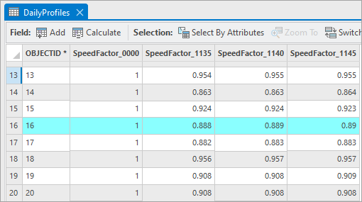
The San Francisco geodatabase in the Network Analyst tutorial data has profiles that cover the day in 5-minute time slices. The SpeedFactor_0000 field contains the free-flow scale factors for midnight to 12:05 a.m. The SpeedFactor_1140 field contains the multipliers for 11:40 a.m. to 11:45 a.m. When a street feature is related to a profile, you can get its expected travel time for any time of the day. For example, if a street is related to profile 16, which is shown in the following image, you can calculate the expected travel time at 11:41 a.m. by multiplying the street's free-flow travel time with the profile's SpeedFactor_1140 value (0.889).
Streets-Profiles table
The Streets-Profiles table identifies street features, their free-flow travel speeds (or travel times), and their related traffic profiles for each day of the week. The following table lists the required fields, an example field name, their allowed data types, and a short description:
| Field | Field name example | Data type | Description |
|---|---|---|---|
Edge feature class identifier | EdgeFCID You must name this field EdgeFCID. | Long integer | Identifies the feature class that stores the street feature. |
Edge feature identifier | EdgeFID You must name this field EdgeFID. | Long integer | Identifies the street feature. |
Edge from position | EdgeFrmPos You must name this field EdgeFrmPos. | Double | Works in conjunction with EdgeToPos to identify a direction of travel or side of the street. Zero indicates the beginning of the line feature as defined by its digitized direction. One indicates the opposite end. For example, an EdgeFrmPos value of 0 and an EdgeToPos value of 1 identifies the right side of the line feature (assuming right-hand traffic). The traffic profiles listed in the same record represent traffic for that side of the street only. Any decimal values specify a position along the digitized direction of the feature, which allows the Dissolve Network tool to maintain the proper profiles for streets after edges have been dissolved together. |
Edge to position | EdgeToPos You must name this field EdgeToPos. | Double | Works in conjunction with EdgeFrmPos to identify a direction of travel or side of the street. |
Free-flow Speed Field or Free-flow Travel Time Field | BaseSpeedKPH or FreeflowMinutes | Float or double (Free-flow Travel Time Field) Float or double or short or long integer (Free-flow Speed Field) | The free-flow speed. Optionally, the free-flow travel time. As a free-flow speed field, it can represent kilometers per hour or miles per hour. As a free-flow travel time field, it can represent days, hours, minutes, or seconds. |
Sunday Profile Field | Profile_1 SundayProfile | Short or long integer | The object ID from the Profiles table that best represents the traffic pattern on Sundays for the portion of the street identified by EdgeFCID, EdgeFID, EdgeFrmPos, and EdgeToPos. |
Monday Profile Field | Profile_2 MondayProfile | Short or long integer | The object ID from the Profiles table that best represents Monday traffic. |
Tuesday Profile Field | Profile_3 TuesdayProfile | Short or long integer | The object ID from the Profiles table that best represents Tuesday traffic. |
Wednesday Profile Field | Profile_4 WednesdayProfile | Short or long integer | The object ID from the Profiles table that best represents Wednesday traffic. |
Thursday Profile Field | Profile_5 ThursdayProfile | Short or long integer | The object ID from the Profiles table that best represents Thursday traffic. |
Friday Profile Field | Profile_6 FridayProfile | Short or long integer | The object ID from the Profiles table that best represents Friday traffic. |
Saturday Profile Field | Profile_7 SaturdayProfile | Short or long integer | The object ID from the Profiles table that best represents Saturday traffic. |
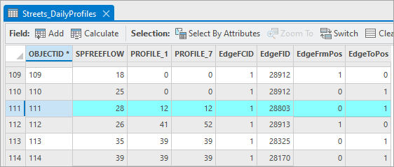
An example of a Streets-Profiles table is the table entitled Streets_DailyProfiles in the following screen shot. The field, PROFILE_1, represents Sunday Profile Field; PROFILE_7 represents Saturday Profile Field; and PROFILE_2 through PROFILE_6 (not shown) represent the Monday through Friday Profile Fields.
The selected record (ObjectID 111) relates profiles for each day of the week with the from-to side of the street feature that has an object ID of 28803. The from-to direction of the street is identified by the EdgeFrmPos and the EdgeToPos values, which are respectively zero and one. Traffic profile 12 represents that side of the street on Sundays and Saturdays, since 12 is the value in the PROFILE_1 and PROFILE_7 fields. The SPFREEFLOW field indicates the travel speed for the street in the from-to direction under free-flow conditions.
The first record (Object ID 109) stores the profiles for a street segment in the to-from direction, and the second record (Object ID 110) stores them for the same street segment in the opposite direction. This is inferred from the EdgeFCID and EdgeFID values, which are identical, and the EdgeFrmPos and EdgeToPos values, which are reversed. Notice that their Sunday and Saturday Profile Field values are zero. This means data wasn't collected or a profile wasn't chosen for those days. When evaluating Saturday or Sunday historical travel times for that edge, the evaluator will need to fall back to a secondary cost attribute defined in the edge traffic evaluator.
Modify historical traffic
Follow the steps below to modify a network's historical traffic settings:
- Open the Network Dataset Properties dialog box.
- Click Traffic.
Two tabs, Historical Traffic and Live Traffic, appear. However, if the network dataset you're using was not configured to support traffic at the time it was created, these tabs will be unavailable.
- Click the Historical Traffic tab.
- Specify whether your historical traffic data is based on speed or travel time.
Traffic profiles based on travel time must have values of 1 or greater, since 1 represents free-flow times and any scale factor larger than that indicates longer travel times. In contrast, when profiles are based on travel speeds, the scale factors must be between 0 and 1, with 1 representing free-flow traffic speeds. As the scale factor approaches zero, the speeds also approach zero.
- Set the properties in the Traffic Profiles section.
- Set the properties in the Profile Assignment section.
- Click OK.
Changes are saved to the network dataset.