The Weighted Overlay tool applies one of the most used approaches for overlay analysis to solve multicriteria problems such as site selection and suitability models. In a weighted overlay analysis, each of the general overlay analysis steps is followed.
As with all overlay analysis, in weighted overlay analysis, you must define the problem, break the model into submodels, and identify the input layers.
Since the input criteria layers will be in different numbering systems with different ranges, to combine them in a single analysis, each cell for each criterion must be reclassified into a common preference scale such as 1 to 10, with 10 being the most favorable. An assigned preference on the common scale implies the phenomenon's preference for the criterion. The preference values are on a relative scale. That is, a preference value of 10 is twice as preferred as a preference value of 5.
The preference values should not only be assigned relative to each other within the layer but also have the same meaning between the layers. For example, if a location for one criterion is assigned a preference of 5, it will have the same influence on the phenomenon as a 5 in a second criterion.
In a simple housing suitability model, you may have three input criteria: slope, aspect, and distance to roads. The slopes are reclassed on a scale of 1 to 10, with the flatter being less costly; therefore, they are the most favorable and are assigned the higher values. As the slopes become steeper, they are assigned decreasing values, with the steepest slopes being assigned a 1. You do the same reclassification process to the 1-to-10 scale for aspect, with the more favorable aspects—in this case, the more southerly—being assigned the higher values. The same reclassification process is applied to the distance to roads criterion. The locations closer to the roads are more favorable since they are less costly to build on, because they have easier access to power and require shorter driveways. A location assigned a suitability value of 5 on the reclassed slope layer will be twice as costly to build on as a slope assigned a value of 10. A location assigned a suitability of 5 on the reclassed slope layer will have the same cost as a 5 assigned on the reclassed distance to roads layer.
Each of the criteria in the weighted overlay analysis may not be equal in importance. You can weight the important criteria more than the other criteria. For instance, in our sample housing suitability model, you might decide that because of long-term conservation purposes, the better aspects are more important than the short-term costs associated with the slope and distance to roads criteria. Therefore, you may weight the aspect values as twice as important as the slope and distance to roads criteria.
The input criteria are multiplied by the weights and then added together. For example, in the housing suitability model, aspect is multiplied by 2 and the three criteria are added together, or represented another way, (2 * aspect) + slope + distance to roads.
The final step of the overlay analysis process is to validate the model to make sure that what the model indicates is at a site is actually there. Once the model is validated, a site is selected and the house is built.
Using the Weighted Overlay tool
The Weighted Overlay tool lets you implement several of the steps in the general overlay analysis process within a single tool.
The tool combines the following steps:
- Reclassifies values in the input rasters into a common evaluation scale of suitability or preference, risk, or some similarly unifying scale
- Multiplies the cell values of each input raster by the raster's weight of importance
- Adds the resulting cell values together to produce the output raster
The tool only accepts integer rasters as input, such as a raster of land use or soil types. Continuous (floating-point) rasters must be reclassified to integer before they can be used.
Generally, the values of continuous rasters are grouped into ranges, such as for slope, or Euclidean distance outputs. Each range must be assigned a single value before it can be used in the Weighted Overlay tool. The Reclassify tool allows for such rasters to be reclassified. You can either leave the value assigned to each range (but note the range of values to which the new value corresponds) and assign weights to the cell values in the Weighted Overlay tool later, or you can assign weights at the time of reclassifying. With the correct evaluation scale chosen, add the raster to Weighted Overlay. The cells in the raster will already be set according to suitability or preference, risk, or some similarly unifying scale. The output rasters can be weighted by importance and added to produce an output raster.
If the Weighted Overlay tool was used for suitability modeling (to locate suitable areas), higher values generally indicate that a location is more suitable. If the tool was used to generate a cost surface (to find out how much it will cost to travel through the landscape, for instance), high values generally indicate higher travel costs. You must understand the scale values you apply to input rasters so you know what the values in the output raster mean.
Running the Weighted Overlay tool
The steps for running the Weighted Overlay tool are as follows:
- Select an evaluation scale.
The evaluation scale represents the range of suitability (or other criterion); the values at one end of the scale represent one extreme of suitability (or other criterion), and values at the other end represent the other extreme.
The default evaluation scale is from 1 to 9 in increments of 1 (for example, with least suitable being 1 and most suitable being 9). If your input rasters are already reclassified to a common measurement scale using the Reclassify tool, it is important to select an evaluation scale that matches the scale used when reclassifying. For instance, if rasters were reclassified using a scale of 1 to 10 (1 being least suitable and 10 being most suitable), an evaluation scale of 1 to 10 by increments of 1 should be entered for the evaluation scale in Weighted Overlay.
- Add input rasters.
Select layers from the map content or browse for raster datasets on file using the (v) or (+) icons, respectively, on the input weighted overlay table. Select a raster row in the table and change the field if desired. Click the Add Raster button again to enter the next raster, and so on.
Note:
If land use is one of your inputs, you might have a description field that describes each land-use type. Using this field instead of the default value field makes it easier to assign weights to this raster.
Note:
Only discrete integer rasters can be used. Reclassify continuous rasters before adding them to Weighted Overlay.
- Set scale values.
The cell values for each input raster in the analysis are assigned values from the evaluation scale. This makes it possible to perform arithmetic operations on rasters that originally held dissimilar types of values. You can change the default values assigned to each cell according to importance or suitability. For instance, a land-use raster that is added has values representing the land-use type (Forest = 7, Water = 3, Barren land = 1, Scrub land = 10). To find suitable locations on which to build, you would assign scale values depending on which land-use types are more suitable. For example, with an evaluation scale set at 1 to 9 by 1, you might assign the following scale values: Forest = 3, Water = Restricted, Barren land = 9, Scrub land = 7.
- Assign weights to input rasters.
Each input raster can be weighted, or assigned a percentage influence, based on its importance. The total influence for all rasters must equal 100 percent. For instance, it might be more important to build a shopping center on soils that are stable than to locate in a popular shopping area.
- Run the Weighted Overlay tool.
The cell values of each input raster are multiplied by the raster's weight (or percent influence). The resulting cell values are added to produce the final output raster.
Using Restricted and NoData for the scale value
Setting a scale value to Restricted assigns a value to that cell in the output weighted overlay result that is the minimum value of the evaluation scale set, minus 1. If there are no inputs to Weighted Overlay with cells of NoData, you could use NoData as the scale value to exclude certain values. However, it is safest, and essential if you have NoData cells in any of your inputs, to use Restricted instead. Potentially, you could have a result from Weighted Overlay that contains cells of NoData that have come from one or more of the inputs (NoData on any input equals NoData in the result) and restricted areas that you purposely excluded. NoData and Restricted values should not be confused. Each serves a specific purpose. There may be areas of NoData where you don't know the value that are actually suitable areas. If you use NoData instead of Restricted to exclude certain cell values, and there is NoData in one or more inputs, you will not know if a cell of NoData means the area is restricted from use or whether there was no input data available in that location.
Take care using Restricted for the scale value when creating a cost surface. Since using Restricted gives a value to the cell that is the minimum value of the evaluation scale, minus 1, your restricted areas will appear to be given the lowest cost, when they are actually excluded from the analysis. Instead, you should assign a high cost or set the scale value to NoData for areas you want excluded from the analysis.
Weighted Overlay tool example
In the following example, a location for a new urban park is being chosen. Three factors will be considered: land use, population density, and distance to existing parks. The goal is to find an area of suitable land use, such as vacant land, in a neighborhood of high population density to provide green space in crowded areas that are not already served by an existing park.
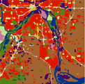
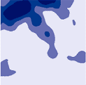
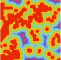
The input rasters to the weighted overlay are displayed in the image above. They are (from left to right) land use, population density, and distance to parks.
The weighted overlay model is displayed in the image below as a process in ModelBuilder:
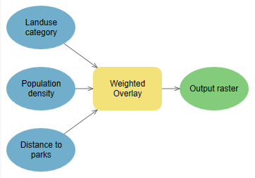
Each value class in each input raster is assigned a new, reclassified value on an evaluation scale of 1 to 5, where 1 represents the lowest suitability and 5 the highest. For instance, in the land-use raster, vacant land is highly suitable, while commercial land is not. In the population density raster, suitability values are high for high-density areas and low for low-density areas. In the distance to parks raster, suitability increases with distance from existing parks because areas far from existing parks are inadequately served.
Any class can also be assigned a Restricted value, which means that the corresponding area is unacceptable or cannot be used. Restricted areas are excluded from the analysis. In the land-use raster, for example, airports and water bodies are restricted.
Each of the three input rasters is then weighted. In this weighted overlay, land use has a 50 percent influence, population density a 15 percent influence, and distance from parks a 35 percent influence.
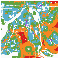
The most suitable areas are shown in red. Orange areas are next, followed by green. Blue and purple areas are least suitable, and white areas are restricted. Modifying the suitability values or the influence percentages will produce different results.