Available with Image Analyst license.
Principal Component Analysis (PCA) is a classical technique used in exploratory data analysis. It is often used to reduce the dimensionality of the dataset so you can identify features and patterns of the data. For example, in multivariate analysis, PCA can be used to identify which variables are necessary and which variables can be excluded without affecting the analysis result. In multispectral and hyperspectral image analysis, the Multidimensional Principle Components tool can be used to compute a set of principal components that capture most of the information and allow analysis to be performed on a reduced number of bands. Image time series data has become more common but poses challenges to identify and extract targeted information. This tool uses the PCA technique to analyze time series data or multidimensional raster data.
Principal component analysis of multidimensional raster data
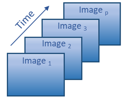
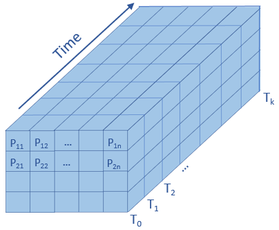
A multidimensional raster contains one or multiple variables. The Multidimensional Principal Components tool analyzes one variable at a time, a 3D image data cube with either (x,y,time) or (x,y,z), and transforms the image data cube into a set of principal components where variance is maximized so that features and patterns in the data can be identified and extracted. An image data cube can be viewed in two ways: a set of images (slices), each representing an image in time or a set of one dimensional arrays, each representing a pixel time series (temporal profile). In the following example, image time series data is used to describe the functionality, with the understanding that the tool can apply to data with a nontime dimension:


You can apply principal component analysis using the dimension reduction mode and the spatial reduction mode. Processing with these two modes entail two different applications.
- Dimension reduction mode analyzes the data as a set of images. It transforms and reduces the data into a set of images that captures the dominant features and patterns. For example, you can extract water pixels prevalent in an image time series and map the water body changes over time. Dimension reduction mode is often used in image time series analysis of land data, such as an NDVI time series.
- Spatial reduction mode analyzes the data as a set of pixel time series. It identifies principal temporal patterns and associated spatial locations of the temporal patterns. For example, you can extract the interannual temporal patten of El Niño and La Niña events using sea surface temperature data and their locations. This is suitable for analysis of long time series but not high-resolution data.
Multidimensional Principal Components tool example
In the example below, the image time series contains k numbers of images X1, X2, …, Xk, and the calculated principal component is a linear combination of the images expressed as the following:
PC1 = a11X1 + a12X2 + … + a1kXkIts matrix form for all principal components is:
Y = XAwhere:
Y = (PC1, PC2, …, PCk)X = (X1, X2, …, Xk)Matrix A contains coefficients that transform the original data into the principal components. The values of matrix A are called loadings, which describe how much each image contributes to a particular principal component. A large loading indicates that the image has a strong relationship to a particular principal component. The sign of a loading indicates whether an image and a principal component are positively or negatively correlated.
The normalized columns in matrix A are eigenvectors, which specify the orientations of principal components relative to the original images. Eigenvalues computed together with eigenvectors indicate the variances explained by each principal component. Eigenvalues, ordered from largest to smallest, determine the sequence of the principal components.
The first component is calculated so that it accounts for the greatest possible variance in the data, the second component accounts for the next highest variance, with the condition that it is uncorrelated (perpendicular) to the first component, and so on. This continues until the total number of specified components have been calculated. All the information contained in the original data is preserved if you compute all principal components.
See Introduction to Principal Component Analysis (PCA) for more information.
Refer to the Multidimensional Principal Components tool for more details.