The Time Series AI tools in the GeoAI toolbox use deep learning-based Time Series Forecasting models to forecast future values at every location in a space-time cube. These models are trained using the Train Time Series Forecasting Model tool on existing time series data, and trained models can be used for prediction using the Forecast Using Time Series Model tool. The primary output is a map of the final forecasted time step as well as informative messages and pop-up charts. Other explanatory variables can be provided to improve the forecast of the analysis variable.
The tools use different types of deep neural networks for Time Series Forecasting. The supported network architectures include fully connected networks as well as convolutional neural networks and LSTM (long short-term memory) for Time Series Forecasting. The details of the model architectures are described later.
The training data used to train the models is constructed using time windows on each variable of the input time series data. Time series data can follow complex trends and have multiple levels of seasonality. Deep learning-based models have a high capacity to learn and can learn these patterns across different kinds of time series and locations, provided there is enough training data. The training tool trains a single global forecast model that uses training data from each location. This global model is used to forecast future values at every location using the forecasting tool.
Potential applications
Deep learning-based models can learn complex trends in the data, so they are used in many contexts. They are most effective compared to other forecasting methods when the data has complex trends or seasonality, and when there is enough training data available to learn these relationships.
For example, you can use the Time Series AI toolset in the following applications:
- A retail store manager can predict demand for consumer products based on historical sales data and maintain stocks accordingly.
- An epidemiologist can model the rise in infectious diseases and predict the number of patients who would need hospitalization within the next week.
- A wind energy plant can forecast how much wind power will be produced based on historical trends and weather data.
- A property investor can estimate the trends in housing price based on historical data and its relationship with factors such as the lending rate, gold price, and stock market indicators.
- Policy makers can forecast the demand for housing, electricity, and water in urban regions.
- Meteorologists can predict El Niño-Southern Oscillation (ENSO) based on climate variables and indices such as winds and sea surface temperatures over the tropical eastern Pacific Ocean.
Model training and prediction
The Train Time Series Forecasting Model tool is used to train a deep learning-based time series forecasting model on historical data. One or more variables can serve as explanatory variables, and the model uses time slices of historical data across locations to learn the trends, seasonality, patterns, and relationships between past data and the value of the analysis variable at subsequent time steps.
The error (also known as loss) in prediction is used to guide model training using gradient descent. The model gradually improves over several training passes over the entire data (epochs) and computed error (difference between the prediction and the ground truth value at the next time step) goes down as training progresses. By default, the model training stops when the loss of the validation data does not register any improvement after five consecutive epochs, unless the Stop training when model no longer improves parameter is not checked. The trained model is saved as a deep learning package (.dlpk) and can be used for forecasting on unseen time series data using the Forecast Using Time Series Model tool.
Model architectures
The supported model architectures are described below.
LSTM (long short-term memory)
Time series data is temporal or sequential in nature, which can be handled by recurrent neural network (RNNs). RNNs remember past information and pass it on to the current input state. However, ordinary RNNs are not able to remember long-term dependencies due to vanishing gradients. LSTM is an upgraded type of RNN, which solves this problem. LSTM is built of units, each consisting of four neural networks, which are used to update its cell state using information from new inputs and past outputs.
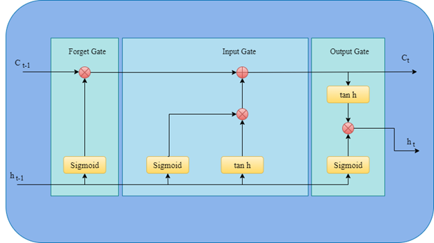
When you choose LSTM as the Model Type parameter value, the following Model Argument can be provided to customize the model when not using the defaults:
| Name | Default value | Description |
|---|---|---|
hidden_layer_size | 100 | The size of the hidden layer |
Fully Convolutional Network (FCN)
Fully Convolutional Networks (FCNs) have mainly been used for images for semantic segmentation and other computer vision problems. They take an image as input and pass it through a series of convolutional layers to extract features of importance. Such neural networks are also able to extract trends and seasonality in time series data and give surprisingly good results for Time Series Forecasting. Given input time series data, a one-dimensional filter slides over it in each convolutional layer to extract time invariant discriminative features with high predictive ability.
Convolutional layers are computationally efficient due to reduced parameters, as local connectivity is provided between the input and output layers. Parameter sharing also significantly reduces the number of required parameters by having the same kernel weight for individual filters. The most prominent benefit of convolutional neural networks is shift invariance, which makes the network robust when detecting important features irrespective of their location within the data.
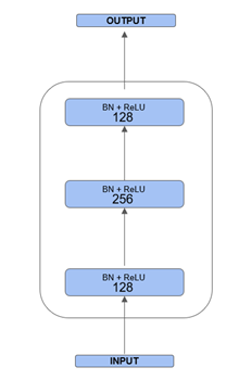
The FCN time series model uses three 1D convolution layers without striding and pooling. Average pooling is done at the last layer of the architecture. After every convolution, batch normalization is performed and rectified linear units (ReLUs) are used asactivation functions. The network architecture is depicted as follows:
InceptionTime
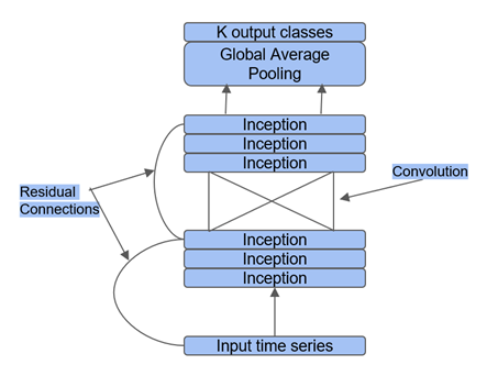
This CNN (convolutional neural network) is based on the previously proposed Inception network "Going Deeper with Convolutions" (2015) [1] for image classification. Before InceptionTime, the computational power of neural networks was based on their depth. The inception module proposed in this paper uses various convolutions in parallel and concatenates their output, thereby increasing both the depth and width of the network, while keeping the computational budget constant.
The InceptionTime model applies this architecture for Time Series Forecasting. In this model, the concatenation is done for one-dimension convolution layers of kernel sizes of length 10, 20, and 40, and a max pooling layer of size 3. Also, a residual connection is introduced at every third inception module, as shown in the following figure. The Inception network also makes heavy use of bottleneck layers, where filters of length 1 and stride 1 are used to reduce the dimensionality of the time series as well as the model complexity, while preventing overfitting. Multiple such inception blocks are used in the network followed by a global average pooling layer.
ResNet
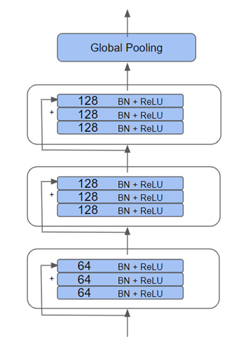
Conventional wisdom with deep neural networks is that the deeper the network is, the better it should perform, as there are more parameters to learn complex tasks. However, it was observed that the model performance actually gets degraded with more depth due to the problem of vanishing gradients. To solve this problem, residual block was introduced in the ResNet architecture. This model is composed of residual blocks, in which skip connections, or shortcut connections, are added. These direct connections allow gradient to flow unhindered to earlier layers of the network along them to learn better.
For Time Series Forecasting, the architecture is adapted in the "Time Series Classification from Scratch with Deep Neural Networks: A Strong Baseline" paper by Wang et. al. 2016. The network uses three residual blocks, as shown in the following figure. Each block contains a combination of three convolutions with batch normalization and uses ReLU as the activation function. Skip connections are added at input and output. The filter sizes used here are of length 64,128, and 128, respectively, and the last layer uses global average pooling.
ResCNN
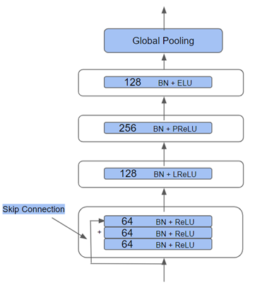
This network is a combination of ResNet and convolution neural networks. A single skip connection is added to the network for better information transfer. To solve overfitting due to skip connections in all the residual blocks, this architecture uses skip a connection in the first block only, as shown in the following figure. Diversified activation functions, including ReLU, LReLU, PReLU, and ELU, are used at different layers to achieve a decent abstraction [2].
TimeMoE
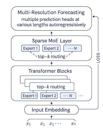
The Time-MoE architecture is a scalable, decoder-only transformer framework designed specifically for time series forecasting. It incorporates a Mixture-of-Experts (MoE) mechanism, where only a subset of its large parameter space is activated during inference, enabling efficient computation and specialization across diverse forecasting tasks. The model supports long input sequences (up to 4,096 time steps) and arbitrary prediction horizons, making it highly flexible. It uses gated MLP-based input embeddings tailored for time series data and rotary positional embeddings (RoPE) for temporal encoding. The architecture is fully trainable, allowing researchers and practitioners to fine-tune it on domain-specific datasets or train it from scratch, offering full control over model design, expert routing, and training configurations.
Forecasting and validation
To ascertain how well the model is performing, the tool relies on two metrics. The first is the forecast metric and the second is the validation metric. The forecast metric provides a way of telling how well the forecast fits the existing data, and the validation metric provides information on how well the model forecasts the validation data that is set aside while the model is trained.
- Forecast metric
The tool trains a single model by combining the data from different locations of a space time cube and the model learns the salient features of the data at each location. The trained model is then used to forecast at future time slices. The fit of the model on the existing training data is measured using forecast root mean square error (RMSE), which is equal to the square root of the average squared difference between the values learned by the model and the actual values of the time series.

Where T is the number of time steps, ct is value learned by the model, and rt is the raw value of the time series at time t.
The following image shows the raw values of a time series along with the values learned by the time series model. The Forecast RMSE measures how much these two time series differ.
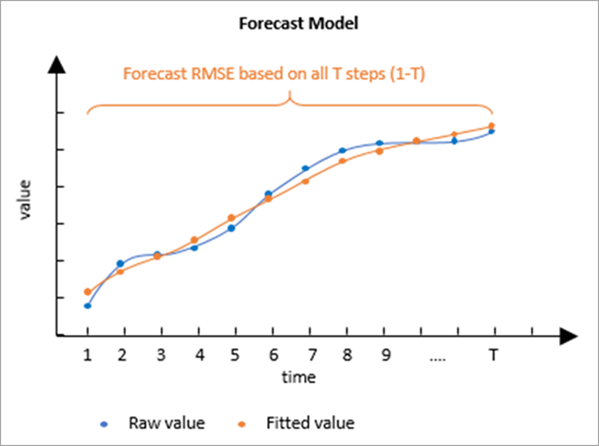
The Forecast RMSE only measures how well the curve fits the raw time series values. It does not measure how well the trained model forecasts future values. It is common for a model to fit a time series closely but not provide accurate forecasts when extrapolated, and hence validation RMSE is a more reliable metric.
- Validation metric
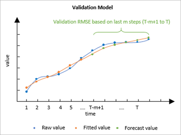
The validation model is used to determine how well the forecast model can forecast future values of each time series. It is constructed by excluding some of the final time steps of each time series and training the model with the data that was not excluded. This model is then used to forecast the values of the data that was withheld, and the forecasted values are compared to the raw values that were hidden. By default, 10 percent of the time steps are withheld for validation, but this number can be changed using the Number of Time Steps to Exclude for Validation parameter. The number of time steps excluded cannot exceed 25 percent of the number of time steps, and no validation is performed if 0 is specified. The accuracy of the forecasts is measured by calculating a Validation RMSE statistic, which is equal to the square root of the average squared difference between the forecasted and raw values of the excluded time steps.

Where T is the number of time steps, m is the number of time steps withheld for validation, ct is the value forecasted from the first T-m time steps, and rt is the raw value of the time series withheld for validation at time t.
The following image shows the values fitted by the model to the first half of a time series and extrapolated to forecast the second half of the time series. The Validation RMSE measures how much the forecasted values differ from the raw values at the withheld time steps.
Tool outputs
The primary output of this tool is a 2D feature class showing each location in the Input Space Time Cube symbolized by the final forecasted time step with the forecasts for all other time steps stored as fields. Although each location is independently forecasted and spatial relationships are not taken into account, the map may display spatial patterns for areas with similar time series.
Pop-up charts
Clicking any feature on the map using the Explore navigation tool displays a chart in the Pop-up pane showing the values of the space-time cube along with the fitted values and the forecasted values. The values of the space-time cube are displayed in blue and are connected by a blue line. The fitted values are displayed in orange and are connected by a dashed orange line. The forecasted values are displayed in orange and are connected by a solid orange line representing the forecasting of the forest model. You can hover over any point in the chart to see the date and value of the point.
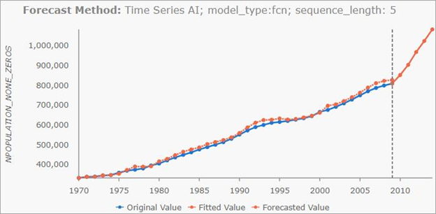
The pop-up chart displays the original values, fitted values, and forecasted values.
Geoprocessing messages
The tool provides a number of messages with information about the tool's run. The messages have three main sections.
The Input Space Time Cube Details section displays properties of the input space-time cube along with information about the number of time steps, number of locations, and number of space-time bins. The properties displayed in this first section depend on how the cube was originally created, so the information varies from cube to cube. The Analysis Details section displays properties of the forecast results, including the number of forecasted time steps, the number of time steps excluded for validation, and information about the forecasted time steps.
The Summary of Accuracy across Locations section displays summary statistics for the Forecast RMSE and Validation RMSE among all of the locations. For each value, the minimum, maximum, mean, median, and standard deviation are displayed.
Note:
Geoprocessing messages appear at the bottom of the Geoprocessing pane during the tool's run. You can access the messages by hovering over the progress bar, clicking the pop-out button  , or expanding the messages section in the Geoprocessing pane. You can also access the messages for a previously run tool using geoprocessing history.
Output fields
In addition to Object ID, geometry fields, and the field containing the pop-up charts, the Output Features will have the following fields.
- Location ID (LOCATION)—The Location ID of the corresponding location of the space-time cube.
- Forecast for (Analysis Variable) in (Time Step) (FCAST_1, FCAST_2, and so on)—The forecasted value of each future time step. The field alias displays the name of the Analysis Variable and the date of the forecast. A field of this type is created for each forecasted time step.
- Forecast Root Mean Square Error (F_RMSE)—The Forecast RMSE.
- Validation Root Mean Square Error (V_RMSE)—The Validation RMSE. If no time steps were excluded for validation, this field is not created.
- Forecast Method (METHOD)—A text field displaying the type of Time Series AI model used and the sequence length.
References
For more information about deep learning-based Time Series Forecasting models, see the following references:
- Szegedy, Christian, Wei Liu, Yangqing Jia, Pierre Sermanet, Scott Reed, Dragomir Anguelov, Dumitru Erhan, Vincent Vanhoucke, and Andrew Rabinovich. "Going deeper with convolutions." In Proceedings of the IEEE conference on computer vision and pattern recognition, pp. 1-9. 2015.
- Ismail Fawaz, Hassan, Benjamin Lucas, Germain Forestier, Charlotte Pelletier, Daniel F. Schmidt, Jonathan Weber, Geoffrey I. Webb, Lhassane Idoumghar, Pierre-Alain Muller, and François Petitjean. "Inceptiontime: Finding alexnet for time series classification." Data Mining and Knowledge Discovery34, no. 6 (2020): 1936-1962.
- Wang, Zhiguang, Weizhong Yan, and Tim Oates. "Time series classification from scratch with deep neural networks: A strong baseline." In 2017 International joint conference on neural networks (IJCNN), pp. 1578-1585. IEEE, 2017.
- Zou, Xiaowu, Zidong Wang, Qi Li, and Weiguo Sheng. "Integration of residual network and convolutional neural network along with various activation functions and global pooling for time series classification." Neurocomputing367 (2019): 39-45.
- Hochreiter, Sepp, and Jürgen Schmidhuber. "Long short-term memory." Neural computation9, no. 8 (1997): 1735-1780.