The concepts covered in this topic apply to the Viewshed and Observer Points tools. The visibility analysis tool Geodesic Viewshed is similar to these, but with some differences in tool behaviors. The Geodesic Viewshed tool takes any numerical fields for observer properties, whereas the Viewshed and Observer Points tools only honors fixed field names (such as OFFSETA, OFFSETB, and so on) from the input observer features attribute table.
A viewshed identifies the cells in an input raster that can be seen from one or more observation locations. Each cell in the output raster receives a value that indicates how many observer points can be seen from each location. If you have only one observer point, each cell that can see that observer point is given a value of 1. All cells that cannot see the observer point are given a value of 0. The observer points feature class can contain points or lines. The nodes and vertices of lines will be used as observation points.
Why calculate viewshed?
The viewshed analysis tools are useful when you want to know how visible objects might be—for example, from which locations on the landscape will the water towers be visible if they are placed in a particular location, or what will the view be from a road?
In the example below, the viewshed from an observation tower is identified. The elevation raster displays the height of the land (lighter shades represent higher elevations), and the observation tower is marked as a green triangle. The height of the observation tower can be specified in the analysis. Cells in green are visible from the observation tower, while cells in red are not.
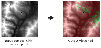
Using the transparency slider, you can display a hillshade raster layer underneath your elevation raster and incorporate the output from viewshed analysis for visualizing the relationship between visibility and terrain.
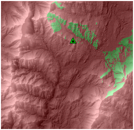
Not only can you determine which cells can be seen from the observation tower, but if you have several observation points, you can also determine which observers can see each observed location. Knowing which observer can see which locations can affect decision making. For example, in a visual quality study for siting a landfill, if it is determined that the proposed landfill can only be seen from dirt roads and not from the primary and secondary roads, it may be deemed a favorable location.
Tools for viewshed and observer points analysis
There are several tools available for visibility analysis. This topic mainly discuss Viewshed and Observer Points. They can both be used to generate an output viewshed raster. The output from Observer Points additionally identifies exactly which observer points are visible from each raster surface location.
Viewshed tool
The Viewshed tool creates a raster, recording the number of times each area can be seen from the input point or polyline observer feature locations. This value is recorded in the VALUE item in the table of the output raster. All cell locations assigned NoData on the input raster are assigned NoData on the output raster.
- When polyline input is used, every node and vertex along each input arc is processed as an individual observation point. The values in the VALUE item of the output raster give the number of nodes and vertices visible to each cell.
- When a SPOT attribute item does not exist in the input observer features table, bilinear interpolation is used to determine the elevation of each observation point. If the nearest raster cell to an observation point or vertex has a NoData value, the tool will be unable to determine its elevation. In this case, the observation point will be excluded from the viewshed analysis.
- Intervening NoData cells between the point of observation and other cells are evaluated as invisible and do not obscure visibility.
Examples of applications for Viewshed
Some examples of the types of questions that can be answered with the Viewshed tool are described in the following table:
| Question | Viewshed options |
|---|---|
Which areas can be seen from a fire lookout tower that is 15 meters high? | Point data, OFFSETA |
How frequently can a proposed disposal site be seen from an existing highway? | Line |
Where should the next communications repeater tower in a series be located? | Point data, OFFSETA, OFFSETB, VERT1, VERT2, AZIMUTH1, AZIMUTH2 |
Viewshed example
An example application of the Viewshed tool is to identify the areas in a study area that can see the towers of a proposed transmission line. The inputs to the analysis are the following:
- A surface elevation raster
- A raster recording the canopy height, which is the height of the top of the vegetation above the ground surface at each location
- A line feature class where the vertex of each line represents the location of the towers that are to support the cable
Step 1: Add the vegetation height raster to the surface elevation raster with the Plus tool.
Input raster or constant value 1 : canopy_height
Input raster or constant value 1 : elev_surface
Output raster : elev_canopy
Step 2: Perform the viewshed analysis within the Viewshed tool.
Input raster : elev_canopy
Input point or polyline observer features : powerline
Output raster : elev_viewshed
Z factor : {default}
Use Earth curvature corrections option : {default}
Refractivity coefficient : {default}
The result of this operation is a viewshed raster.
Observer Points tool
The Observer Points tool stores the binary-encoded information about which observation points can see each raster cell. This information is stored in the VALUE item.
To display all the regions of the raster that can be seen only a particular observer, Observer 3 for example, open the output raster attribute table and select the row where observer 3 (OBS3) equals 1 and all other observers equal 0. The regions of the raster that can be seen only by observer 3 will be highlighted on the map.
To use linear data with Observer Points, convert the line feature class with the Feature Vertices To Points tool in the Data Management > Features toolset. There is a limit of 16 points.
When a SPOT attribute item does not exist in the feature attribute table, bilinear interpolation is used to determine the elevation of each observation point. If the nearest input raster cell to an observation point has the NoData value, the tool will be unable to determine its elevation. In this case, the observation point will be excluded from the visibility analysis.
Intervening NoData cells between the point of observation and other cells are evaluated as invisible and do not obscure visibility.
Observer Points details
Observer Points stores the binary-encoded information about which observation points can see each raster cell. This information is stored in the VALUE item.
To display all the regions of the raster that can be seen only by observer 3, open the output raster attribute table and select the row where observer 3 (OBS3) equals 1 and all other observers equal 0. The regions of the raster that can be seen only by observer 3 will be highlighted on the map.
Raster OBSn items
In addition to the standard items VALUE and COUNT in the raster attribute table, new items will be created corresponding to each observer in the input point dataset. The items are OBS1, OBS2, ..., OBSn, where n is the number of observers. They are defined as follows:
ITEM NAME    WIDTH    OUTPUT    TYPE    N.DEC
OBSn         2        2         B       -
These items record the visibility of each cell by every input point observer features observer. For example, every raster cell that can be seen by observer 8 (featurename# = 8) will contain a value of 1 in the item named OBS8. Cells that cannot be seen by the observation point are assigned a value of 0. Cell locations assigned NoData on the input raster are assigned NoData on the output raster.
You can use the OBSn items to identify those raster cells that can be seen from a specific observation point. This is slightly different from the previous case where a selection was made based on the VALUE parameter. In this case, cells that can be seen by observers 1 and 8 may also be seen by other observers (in which case, they each would have a different value).
For example, to display all areas that can be seen by observation points 1 and 8, open the raster attribute table and select the row where both observer 1 (OBS1) and observer 8 (OBS8) equal 1 and all other observers equal 0.
Quantifying visual quality
The information in the tool output can also be used to perform an analysis of visual quality. For example, you can determine the visual quality of all locations on a surface by positioning an observation point at each significant visual feature within the input raster's extent. Such points might include the city dump, auto salvage yard, local parks, and each of the power transmission towers in the region.
After running Observer Points, use the OBSn item in the output raster's table to select those cell locations that can see each visual feature. Use any of a variety of other tools to accumulate positive or negative scores, depending on each observation point's visual quality and weight. After all observation points have been considered, those cell locations with the best scores will have the best visual quality.
Examples of applications for Observer Points
Some examples of the types of questions that can be answered with the Observer Points tool are described in the following table:
| Question | Observer Points options |
|---|---|
Given a set of locations for fire lookout towers, what is the minimum number of towers required to see the entire study area? | Point data, OFFSETA |
Which locations of the raster can see only the disposal site and transmission tower 3? | Point data |
How can I determine which surface locations have the best view? I want to assign different weights to each landscape feature within a viewshed based on its visual quality. | Point data |
Controlling the visibility analysis
It is possible to limit the region of the raster inspected by specifying various items in the feature attribute dataset, such as observation point elevation values, vertical offsets, horizontal and vertical scanning angles, and scanning distances. There are nine items in total: SPOT, OFFSETA, OFFSETB, AZIMUTH1, AZIMUTH2, VERT1, VERT2, RADIUS1, and RADIUS2.
The image below graphically depicts how a visibility analysis is controlled. The observation point is on the mountain top to the left (at OF1 in the image). The direction of the viewshed is within the cone looking to the right. You can control how much to offset the observation point (for example, the height of the tower), the direction to look, and how high and low to look from the horizon.
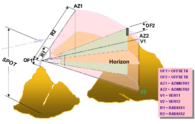
When the observer features dataset is a point feature class, each observation point can have a unique set of observation constraints in the attribute table. When it is a polyline feature class, every vertex along an input polyline uses the same observation constraints contained in the polyline's record in the attribute table.
The definitions for these items can vary as long as they are numeric. Whenever an item does not exist, the default values are applied.
SPOT
The SPOT item is used to define the surface elevations for the observation points.
Offset
The offset is the vertical distance (in surface units) to be added to the z-value of a location on the surface.
There are two offset items, one defining the elevation to be added to the observer location and the other defining what will be added to each cell to be considered for visibility.

OFFSETA
The OFFSETA item indicates a vertical distance in surface units to be added to the z-value of the observation point.
If OFFSETA exists in the feature attribute table, its value is added to the SPOT elevation when present; otherwise, it is added to the interpolated surface z-value. The OFFSETA value must be positive. If the OFFSETA item does not exist, the default value is 1.
OFFSETB
The OFFSETB item indicates a vertical distance in surface units to be added to the z-value of each cell as it is considered for visibility.
If OFFSETB exists in the feature attribute table, its value is added to the surface z-value of each cell location when it is being analyzed for visibility. The value must be positive. If no OFFSETB item is found in the feature attribute table, it defaults to 0.
Azimuth
The azimuth items define the horizontal angle limits to the scan. The sweep proceeds in a clockwise direction from the first azimuth to the second. The values for the angle are given in degrees from 0 to 360, with 0 oriented to north.
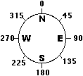
AZIMUTH1
The AZIMUTH1 item defines the start angle of the scan range.
If this item does not exist in the feature attribute table, it defaults to a value of 0.
AZIMUTH2
The AZIMUTH2 item defines the end angle of the scan range. The value for AZIMUTH2 must be greater than that of AZIMUTH1.
If this item does not exist in the feature attribute table, it defaults to a value of 360. If both AZIMUTH1 and AZIMUTH2 are not defined, the defaults will give a full 360° sweep.
Vertical angle
The vertical angle defines the vertical angle limits to the scan. The angles are expressed in degrees between 90 and -90, with positive values representing angles above the horizontal plane and negative angles below. The horizontal plane (0 degrees) is defined by the z-value of the observation point plus the value of OFFSETA. Both vertical angles can be negative.

VERT1
The VERT1 item defines the upper horizontal angle limit of the scan.
If this item does not exist in the feature attribute table, it defaults to a value of 90.
VERT2
The VERT2 item defines the lower horizontal angle limit of the scan. The value for VERT2 must be less than that of VERT1.
If this item does not exist in the feature attribute table, it defaults to a value of -90.
Radius
The radius items limit the search distance when identifying areas visible from each observation point. Cells that are beyond a certain distance can be excluded from the analysis.
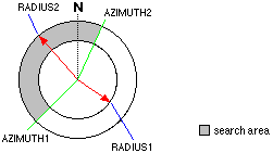
RADIUS1
The RADIUS1 item defines the start distance from which visibility is determined. Note that cells closer than the RADIUS1 search distance are not visible in the output raster, but they can still block the visibility of cells between RADIUS1 and RADIUS2.
The default RADIUS1 distance is 0.
RADIUS2
Cells beyond the RADIUS2 search distance are excluded from the analysis. The value for RADIUS2 should be greater than RADIUS1.
The default RADIUS2 distance is infinity.
Planimetric versus three-dimensional distance
By default, the limiting distances RADIUS1 and RADIUS2 are interpreted as three-dimensional line-of-sight distances. To ensure that the slope distance is calculated correctly, both the ground units and surface z-units must be in the same unit of measure. To process RADIUS1 and RADIUS2 as two-dimensional planimetric distances, insert a negative sign (-) in front of the values.
For example, if RADIUS1 is set to -1000 and RADIUS2 is set to -9000, Viewshed analyzes the regions of the surface between 1,000 and 9,000 ground units measured planimetrically from the observer.
Default settings
The following table shows the default settings for the options that control the visibility analysis:
| Option | Default setting |
|---|---|
SPOT | Estimated using bilinear interpolation |
OFFSETA | 1 |
OFFSETB | 0 |
AZIMUTH1 | 0 |
AZIMUTH2 | 360 |
VERT1 | 90 |
VERT2 | -90 |
RADIUS1 | 0 |
RADIUS2 | Infinity |
Curvature and refraction corrections
Use the earth curvature correction option to correct for the curvature of the earth and refraction. Corrections are made when projection information for the surface is present. In addition, the ground units and surface z-units must be in feet, meters, or units/meter. The formula used for the correction is as follows:
                      Dist2               Dist2
 Zactual = Zsurface - --------- + Rrefr * ---------
Diamearth Diamearth- where:
Dist: The planimetric distance between the observation feature and the observed location.
Diam: The diameter of the earth.
Rrefr: The refractivity coefficient of light.
The default value for the diameter of the earth (Diamearth) is defined as 12,740,000 meters. The default value for the refractivity coefficient (Rrefr) is 0.13, which is based on the Gaussian refraction coefficient (Brunner, F. K., 1984). Different values for Rrefr can be used to factor in variations in atmospheric conditions on visibility.
References
Brunner, F. K. (1984), Geodetic Refraction: Effects of Electromagnetic Wave Propagation Through the Atmosphere. Springer, Berlin