Contours are lines that connect locations of equal value in a raster dataset that represents continuous phenomena such as elevation, temperature, precipitation, pollution, or atmospheric pressure. The line features connect cells of a constant value in the input. Contour lines are often generally referred to as isolines but can also have specific terms depending on what is being measured. Some examples are isobars for pressure, isotherms for temperature, and isohyets for precipitation.
The distribution of the contour lines shows how values change across a surface. Where there is little change in a value, the lines are spaced farther apart. Where the values rise or fall rapidly, the lines are closer together.
The contour creation tools, Contour, Contour List and Contour with Barriers, are used to create a polyline feature dataset from an input raster.
Why create contours?
By following the polyline of a particular contour, you can identify which locations have the same value. Contours are also a useful surface representation, because they allow you to simultaneously visualize flat and steep areas (distance between contours) and ridges and valleys (converging and diverging polylines).
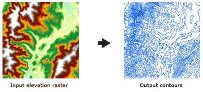
The example below shows an input elevation dataset and the output contour dataset. The areas where the contours are closer together indicate the steeper locations. They correspond with the areas of higher elevation (in white on the input elevation dataset).

The contour attribute table contains an elevation attribute for each contour polyline.
Example showing how contours are created
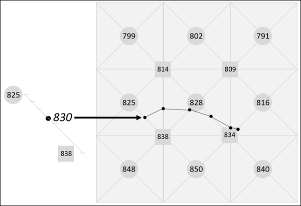
To understand how contour lines are created, consider the example of a raster of nine cells, with the values at the cell centers as shown below, for which you want to create a contour line for an elevation of 830 meters. The first step is to use bilinear interpolation to calculate a central value for each group of four adjacent cells. For the group of four cells at the upper left, this value is calculated as follows: (799 + 802 + 825 + 828) / 4 = 813.5, which is then rounded to 814. Once that is done, the values of the existing cell centers and the new intersection locations are used to determine the path of particular contour values. To create the 830 contour, linear interpolation between the points is used to determine where that value falls along the appropriate vertical, horizontal, and diagonal lines. The contour line is constructed by joining these intersection points.
Extrapolation is not used to interpolate the outer corner values, and therefore the contour lines do not extend to the edge of the raster.

Contour quality
The contour tools produce high-quality contours, representing an exact interpretation of the raster surface. Overall contour accuracy depends on how well the data used to create the input raster represents the actual surface.
The size of the raster cells used affects the appearance of the output contours. A large cell size may result in coarse, blocky contours.
Occasionally, contours may cross, appear to intersect, or form an unclosed branching line. Crossing contours can occur in saddle regions that lie exactly on a contour interval. In other cases, the contours may pass so close to one another that they appear to intersect. Branching contours can occur in cases of intersecting ridges that fall exactly on a contour interval. These are all valid interpretations of the surface that cartographers typically modify for aesthetic purposes.
Controlling contour quality
Occasionally, contours may be created that have square or blocky outlines, appearing to follow raster cell boundaries. This can occur when the raster values are integers and they fall exactly on a contour. This is not a problem, merely an exact contouring of the data.
If you want smoother contours, some ways to overcome this condition include smoothing the source data or adjusting the base contour.
Smoothing the data
Use the ArcGIS Spatial Analyst extension license, The easiest smoothing approach is to preprocess the input raster with the Focal Statistics tool, using the Mean statistic.
Another method is to slightly adjust z-values so a contour will no longer pass exactly through the cell centers of the raster. Again, the Focal Statistics tool is used, but with a custom weighted kernel file and the Sum statistic instead. The structure of the kernel file is as follows:
3 3
.005 .005 .005
.005 .960 .005
.005 .005 .005
The accuracy of the contour will not be significantly affected because the z-value adjustment is small and heavily weighted in favor of the center raster cell.
Adjusting the base contour
Adjusting the base contour involves offsetting the base contour such that the contours no longer pass exactly through the cell centers. The offset can be very small; values as small as 0.0001 have been effective.
Note:
To apply this technique to the Contour List tool, adjust the values in the contour list. For example, instead of 600, 650, 700, and so on, use 600.001, 650.001, 700.001, and so on.
Data issue with USGS DEMs
Legacy:
Tests have revealed that contours generated from rasters created from some older United States Geological Survey (USGS) 7.5-minute digital elevation models (DEMs) may not have the same level of detail as exhibited on the corresponding map sheet available from USGS. This appears to be a factor of the sampling interval inherent in the DEM. USGS 7.5-minute DEMs are sampled at 30-meter intervals, while the contours on the map sheets appear to have been digitized directly from stereo models at a much higher level of detail. The newer SDTS format DEMs from the USGS do not have this problem.