The Aspect tool identifies the direction the downhill slope faces.
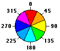
The values of each cell in the output raster indicate the compass direction the surface faces at that location. It is measured clockwise in degrees from 0 (due north) to 360 (again due north), coming full circle. Flat areas having no downslope direction are given a value of -1.
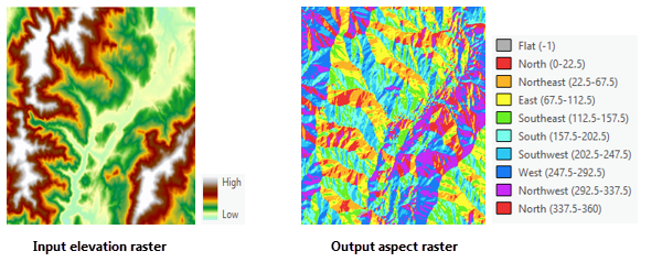
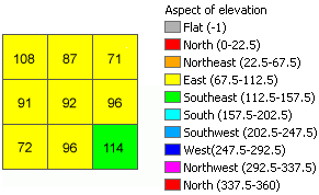
The following images show an input elevation dataset and the output aspect raster.
Note:
The Surface Parameters tool provides a newer implementation of aspect and is recommended to be used instead of the Aspect tool. The Aspect tool fits a plane to the nine local cells, but a plane may not be a good descriptor of the landscape and may mask or exaggerate natural variations of interest. The Surface Parameters tool fits a surface to the neighborhood of cells instead of a plane, which provides a more natural fit to the terrain.
The Aspect tool uses a 3-by-3 window of cells to compute the value, while the Surface Parameters tool allows window sizes from 3-by-3 to 15-by-15 cells. Larger window sizes are useful with high resolution elevation data to capture land surface processes at an appropriate scale. The Surface Parameters tool also provides an adaptive window option that evaluates the local variability of the terrain and identifies the largest appropriate neighborhood size for each cell. This can be useful with gradual homogeneous terrain interrupted by streams, roads, or sharp breaks in slope.
You can continue to use the traditional approach of the Aspect tool if you need the results to exactly match previous tool runs or if fast processing time is more important than a better algorithm.
With the Aspect tool, you can do the following:
- Find all north-facing slopes on a mountain as part of a search for the best slopes for ski runs.
- Calculate the solar illumination for each location in a region as part of a study to determine the diversity of life at each site.
- Find all southerly slopes in a mountainous region to identify locations where the snow is likely to melt first as part of a study to identify those residential locations likely to be hit by runoff first.
- Identify areas of flat land to find an area for a plane to land in an emergency.
Calculation methods and the edge effect
Two methods are available for aspect computation. You can choose between performing Planar or Geodesic calculations with the Method parameter.
With the planar method, the computation will be performed on a projected flat plane using a 2D Cartesian coordinate system. With the geodesic method, the calculation will be performed in a 3D Cartesian coordinate system by considering the shape of earth as an ellipsoid.
Both planar and geodesic computations are performed using a 3 by 3 cell neighborhood (moving window). For each neighborhood, if the processing (center) cell is NoData, the output will be NoData. The computation also requires that at least seven cells neighboring the processing cell have valid values. If there are fewer than seven valid cells, the calculation will not be performed, and the output at that processing cell will be NoData.
The cells in the outermost rows and columns of the output raster will be NoData. This is because along the boundary of the input dataset, those cells do not have enough valid neighbors.
Planar method
The planar method is the traditional method for calculating aspect.
Planar aspect algorithm
A moving 3 by 3 window visits each cell in the input raster, and for each cell in the center of the window, an aspect value is calculated using an algorithm that incorporates the values of the cell's eight neighbors. The cells are identified as letters a to i, with e representing the cell for which the aspect is being calculated.
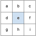
The rate of change in the x direction for cell e is calculated with the following algorithm:
[dz/dx] = ((c + 2f + i)*4/wght1 - (a + 2d + g)*4/wght2) / 8- where:
wght1 and wght2 are the horizontal weighted counts of valid cells.
For instance:
- if c, f, and i all have valid values, wght1 = (1+2*1+1) = 4.
- if i is NoData, wght1 = (1+2*1+0) = 3.
- if f is NoData, wght1 = (1+2*0+1) = 2.
Similar logic applies to wght2, except the neighbor locations are a, d, and g.
The rate of change in the y direction for cell e is calculated with the following algorithm:
[dz/dy] = ((g + 2h + i)*4/wght3 - (a + 2b + c)*4/wght4 ) / 8- where:
wght3 and wght4 are the same concept as in the [dz/dx] computation.
Taking the rate of change in both the x and y direction for cell e, aspect is calculated using the following:
aspect = 57.29578 * atan2 ([dz/dy], -[dz/dx])The aspect value is then converted to compass direction values (0-360 degrees), according to the following rule:
  if aspect < 0
    cell = 90.0 - aspect>
  else if aspect > 90.0
    cell = 360.0 - aspect + 90.0
  else
    cell = 90.0 - aspect
Planar aspect calculation example
As an example, the planar aspect value of the center cell of the moving window will be calculated.
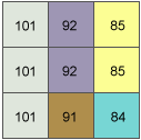
The rate of change in the x direction for the center cell e is:
  [dz/dx] = ((c + 2f + i)*4/wght1 - (a + 2d + g)*4/wght2) / 8
          = ((85 + 170 + 84)*4/(1+2+1) - (101 + 202 + 101)*4/(1+2+1)) / 8
          = -8.125
The rate of change in the y direction for cell e is:
  [dz/dy] = ((g + 2h + i)*4/wght3 - (a + 2b + c)*4/wght4) / 8
          = ((101 + 182 + 84)*4/(1+2+1) - (101 + 184 + 85)*4/(1+2+1)) / 8
          = -0.375
The aspect is calculated as:
  aspect = 57.29578 * atan2 ([dz/dy], -[dz/dx])
         = 57.29578 * atan2 (-0.375, 8.125)
         = -2.64
Since the calculated value is less than zero, the final rule will be applied as:
  cell = 90.0 - aspect
       = 90 - (-2.64)
       = 90 + 2.64
       = 92.64
The value of 92.64 for the center cell e indicates that its aspect is in the easterly direction.
Geodesic method
The geodesic method measures surface aspect in a geocentric 3D coordinate system—also called the Earth Centered, Earth Fixed (ECEF) coordinate system—by considering the shape of the earth as an ellipsoid. The computation result will not be affected by how the dataset is projected. It will use the z-units of the input raster if they are defined in the spatial reference. If the spatial reference of the input does not define the z-units, you will need to do so with the z-unit parameter. The geodesic method produces a more accurate aspect than the planar method.
Geodesic coordinate transformation
The earth-centered earth-fixed (ECEF) coordinate system is a 3D right-handed Cartesian coordinate system with the center of the earth as the origin, where any location is represented by x-, y-, and z-coordinates. See the figure below for an example of a target location (T) expressed with geocentric coordinates.
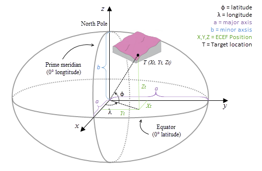
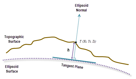
The geodesic computation uses an x-, y-, z-coordinate that is calculated based on its geodetic coordinates (latitude φ, longitude λ, height h). If the coordinate system of the input surface raster is a projected coordinate system (PCS), the raster is first reprojected to a geographic coordinate system (GCS) in which each location has a geodetic coordinate, and is then transformed to the ECEF coordinate system. The height h (z-value) is the ellipsoid height referenced to the ellipsoid surface. See the illustration graphic below.
To transform to ECEF coordinates from a geodetic coordinate (latitude φ, longitude λ, height h), use the following formulas:
X = (N(φ)+h)cosφcosλY = (N(φ)+h)cosφsinλZ = (b2/a2*N(φ)+h)sinφ- where:
- N( φ ) = a2/ √(a2cosφ2+b2sinφ2)
- φ = latitude
- λ = longitude
- h = ellipsoid height
- a = major axis of the ellipsoid
- b = minor axis of the ellipsoid
The ellipsoid height h is in meters in the formulas above. If the input raster's z-unit is specified in any other unit, it will be internally transformed to meter.
Aspect computation
The geodesic aspect at a location is the direction of the downslope surface with respect to north, on a plane that is parallel to the ellipsoid surface.
To calculate the aspect at each location, a 3 by 3 cell neighborhood plane is fitted around each processing cell using the Least Squares Method (LSM). The best fit in the LSM minimizes the sum of squared difference (dzi) between the actual z-value and the fitted z-value. See the illustration below for an example.
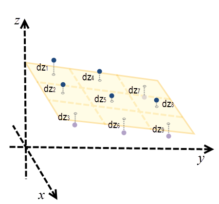
Here, the plane is represented as z = Ax + By + C. For each cell center, dzi is the difference between the actual z-value and the fitted z-value.
The plane is best fitted when ∑9i=1dzi2 is minimized.
After the plane is fitted, a surface normal is calculated at the cell location. At the same location, an ellipsoid normal perpendicular to the tangent plane of the ellipsoid surface is also calculated.
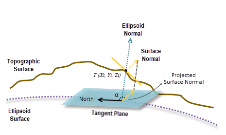
Since the tangent plane of the ellipsoid surface is considered the reference plane, the surface normal is perpendicularly projected onto the plane. Finally, the geodesic aspect is calculated by measuring the angle α in the clockwise direction between the north and the perpendicular projection of the surface normal (see the illustration above).
Should I use the Surface Parameters tool?
If the Input raster parameter value is high resolution with a cell size of less than a few meters, or particularly noisy, consider using the Surface Parameters tool and its user-defined neighborhood distance option instead of the immediate 3-by-3 neighborhood of this tool. Using a larger neighborhood can minimize the effect of noisy surfaces. Using a larger neighborhood can also better represent landforms and surface characteristics when using high resolution surfaces.
Use of a GPU
For the geodesic method, this tool can deliver increased performance if you have certain GPU hardware installed on your system. See the GPU Processing with Spatial Analyst section for details on how this is supported, how to configure it, and how to enable it.
References
Marcin Ligas, and Piotr Banasik, 2011. Conversion between Cartesian and geodetic coordinates on a rotational ellipsoid by solving a system of nonlinear equations (GEODESY AND CARTOGRAPHY), Vol. 60, No 2, 2011, pp. 145-159
E.J.Krakiwsky, and D.E.Wells, 1971. Coordinate Systems In Geodesy (GEODESY AND GEOMATICS ENGINEERING, UNB), LECTURE NOTES, No16, 1971, pp. 18-38
Lancaster, P. and Šalkauskas, K. 1986. Curve and Surface Fitting: An Introduction. London: Academic Press
B. Hofmann-Wellenhof, H. Lichtenegger and J. Collins, 2001. GPS - theory and practice. Section 10.2.1. p. 282.
David Eberly 1999. Least Squares Fitting of Data. (Geometric Tools, LLC), pp. 3.