The Prepare Data for Prediction tool facilitates the splitting of input features to create predictive models. The tool extracts information from explanatory variables, distance features, and explanatory rasters to make the train-test split. It also allows for resampling of original data to account for imbalances in the data. Balancing data is helpful to improve model performance when predicting rare case events.
The objective in predictive modeling is to capture as many underlying patterns as possible while ensuring the model can generalize effectively to new data in the future. Predictive models rely on input data for learning. This input data is called training data. When building a model and training it on the input data, the goal is to achieve a general fit that captures the underlying patterns in the training data while maintaining great predicting performance on unseen, new data. The goal is not to replicate the training data perfectly, which will lead to overfitting. At the same time, we want to avoid being excessively general, which can result in underfitting and missing key patterns in the data.
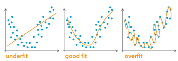
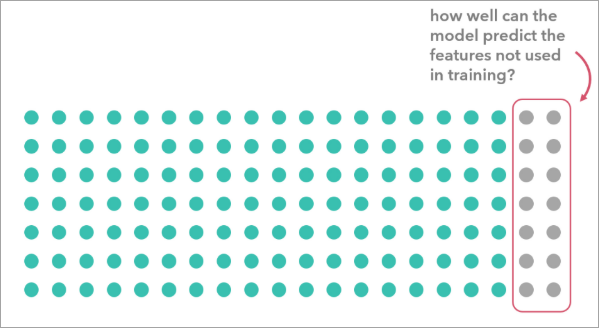
When developing a predictive model, we want to ensure that it performs well on unseen data. Achieving a good fit includes evaluating the model against reserved data where the true values of the predicted variable are known. This allows us to assess the model's performance on unknown data using various metrics. The reserved data containing these true values is commonly referred to as test data or validation data. Typically, the test data is separated from the training dataset and reserved specifically for model evaluation. The Prepare Data for Prediction tool facilitates the process of splitting input features into train-test sets for better model training.
Splitting the data
Splitting data into training and testing data subsets is a best practice when training and evaluating predictive models.
This tool offers the following Splitting Type parameter options to split the data:
- Random Split—A testing subset is selected randomly and therefore is dispersed spatially throughout the study area.
- Spatial Split—A spatial testing subset is spatially contiguous and is separate from the training subset. The spatial split is generated by randomly selecting a feature and identifying its K nearest neighbors in the geographic space. The benefit of using a spatial testing subset is that the testing data will emulate a future prediction dataset that is not in the same study area as the training data.
Data leakage
It is important to be thoughtful when selecting your training data due to potential data leakage. Data leakage occurs when the training data contains information that the model won’t have access to during future predictions. This can lead to a significant overestimation of the model's predictive capabilities. For example, if you use data from delays and cancellations in the afternoon of a specific date to model airline delays, then predict delays and cancellations from the morning of the same day, the model will struggle when deployed in the real world. It's crucial to train your model solely on data that will be available at the time and in the space when making predictions.
Data leakage may also occur due to spatial autocorrelation. For example, neighboring census tracts are likely to exhibit similarities due to spatial autocorrelation. When a model learns from one census tract and tests on its neighbor, it will likely perform reasonably well. However, when predicting to census tracts in a different state, the model's performance may decline significantly. This is because the training data contains information from one area, but the prediction dataset lacks similar information from the different state. To mitigate data leakage due to spatial proximity, set the Splitting Type parameter to Spatial split. You can create a spatial train-test split before training using the Prepare Data for Prediction tool or evaluate various spatial splits with the Evaluate Predictions with Cross Validation tool.
Working with imbalanced data
Imbalanced data refers to a dataset where the distribution is skewed or disproportionate. In the context of classification tasks, imbalanced data occurs when one class (the minority class) has significantly fewer features than other classes (the non-minority classes). This imbalance can lead to challenges in training machine learning models effectively. For example, in a binary classification problem where we predict whether a wildfire will occur, if 99 percent of the features indicate no wildfire (majority class) and only 1 percent indicate a wildfire (minority class), the data is imbalanced. This challenge manifests in the model's results as a low sensitivity for those rarer categories, indicating that the model struggles to correctly identify many features associated with them. For instance, if you're predicting which counties will have a rare disease or identifying individuals committing fraud, accurately recognizing those rare categories becomes crucial, as they are often the most important cases for addressing the issue at hand. If the model cannot learn the patterns in all classes effectively, it could lead to poor generalization to new data and a less effective model.
In a spatial context, imbalanced data may result from the sampling bias. This can result in training samples that have clear spatial clusters that do not accurately represent the entire population. For example, data collection surveys often focus on areas near roads, paths, and other easily accessible locations, introducing inaccuracies into the model and potentially biased conclusions. This tool offers several balancing method options to resample the data and prevent these issues.
Balancing methods
The Balancing Type parameter balances the imbalanced Variable to Predict parameter value or reduces the spatial bias of the Input Features parameter value.
Note:
If the Splitting Type parameter is set to Random Split or Spatial Split, the balancing method is applied only to the output features in the training data. This approach ensures that the test features remain in their original, unaltered form for validation, helping to prevent data leakage issues.
The Balancing Type parameter supports the following options to help you prepare the training data:
- Random Undersampling—Random undersampling is a technique used to balance unbalanced data by randomly removing features from the non-minority classes until all classes have an equal number of features.
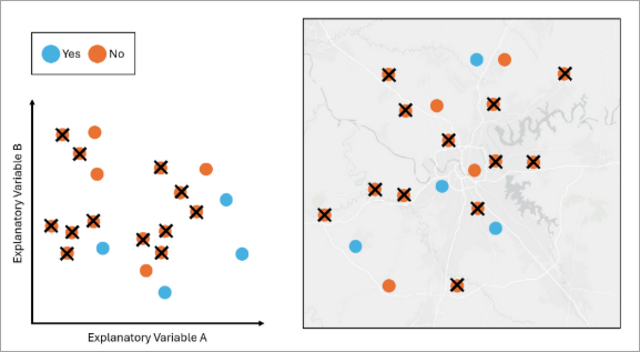
The features in blue are in the minority class and the features in orange are in the non-minority class. If we apply Random Undersampling to the data, the tool will randomly remove the orange features so that the number of orange features matches the number of blue features. - Tomek Undersampling—Tomek’s Link Undersampling is a technique used to balance unbalanced data by removing features from the non-minority classes that are close to the minority class in the attribute space. The purpose of this option is to improve the separation between classes and make a clear decision boundary for a tree-based model such as Random Forest or XG-Boost. This option does not guarantee that all classes have an equal number of features.
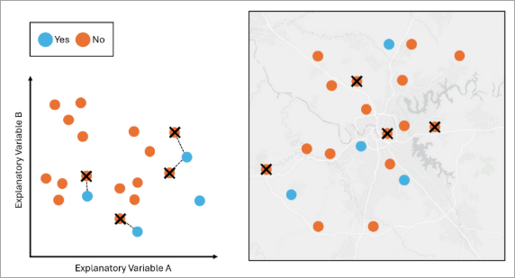
The features in blue are in the minority class, and the features in orange are in the non-minority class. In the variable space, any pair of features from different classes that are nearest neighbors of each other is called Tomek’s Link. If we apply Tomek’s Undersampling to the data, the tool will remove the orange feature if it has a Tomek’s link with a blue feature. - Spatial Thinning—Spatial thinning is a technique to reduce the effect of sampling bias on the model by enforcing a minimum specified spatial separation between features.
When a categorical variable is selected as the variable to predict, the spatial thinning is applied to each group independently to ensure a balanced representation within each category; otherwise, it will be implemented across the entire training dataset regardless of attribute values.
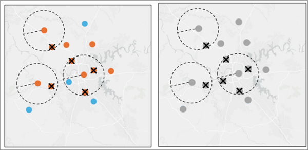
Any features that fall within a designated buffer distance will be removed. - K-medoids Undersampling—K-medoids Undersampling is a technique used to balance unbalanced data by only keeping a number of representative features in the non-minority class so that all classes have an equal number of features. If we apply K-medoids Undersampling to the data, the tool will only keep K features that are medoids in the variable space from the non-minority class. Use K-medoids instead of another clustering algorithm to ensure that there is a central representative preexisting feature from each cluster.
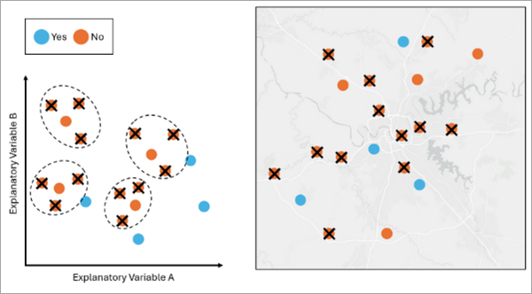
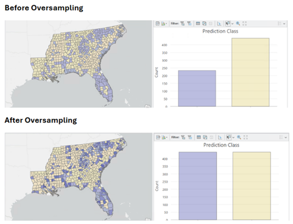
The number of K is equal to the number of features in the minority class, which is 4. The clusters are created within each of the dependent variables’ classes and are clustered based on the values of the explanatory variables. The remaining features in the non-minority class come from the medoid of each cluster. - Random Oversampling—Random Oversampling is a technique used to balance unbalanced data by duplicating randomly selected features in the minority classes until all classes have an equal number of features.
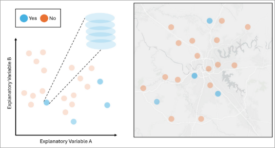
The features in blue are in the minority class, and the features in orange are in the non-minority class. If we apply Random Oversampling to the data, the tool will randomly select and duplicate the blue features so that the number of blue features matches the number of orange features. The variables and the geography of a duplicated feature are the same as the original feature. - SMOTE Oversampling—SMOTE (Synthetic Minority Over-sampling Technique) oversampling is a technique used to balance unbalanced data by generating synthetic features in the minority class until all classes have an equal number of features. A feature in a minority class is chosen, a near feature of the same minority class in the attribute space is selected, and new attributes are generated as an interpolation between those two features. The geometry of the new synthetic feature will be that of the originally selected feature.
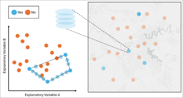
The features in blue are in the minority class, and the features in orange are in the non-minority class. If we apply SMOTE Oversampling to the data, the tool will generate the synthetic features by interpolating the values between two randomly selected features from the minority class in the attribute space. The geography of a synthetic feature is the same as the originally selected feature, while the variables are interpolated from the selected feature.
Best practices
The following are best practices when using this tool:
- It is important to ensure that when using categorical variables as the Variable to Predict or as the Explanatory Variables parameter value, every categorical level appears in the training data. This is important, because the models need to see and learn from every possible category before predicting with new data. If a category appears in the explanatory variables in the testing or validation data that was not in the training data, the model will fail. If a category appears in the Variable to Predict parameter value in the testing or validation data but was not in the training data, the model will be unable to predict that category for any features. The tool will fail if it cannot get all categorical levels in the training dataset after 30 attempted iterations.
- Once data is balanced, it should not be used as validation data or test data, because it no longer represents the distribution of data that will be measured in the real world. Oversampled data should never be used to evaluate model performance as validation data. Undersampled data can be used, however, it is not advised.
- When encoding categorical variables, binary columns (0s and 1s) will be created and added to the attribute tables of the training and testing output features. A 1 indicates presence of the categorical level and 0 represents absence. When using a linear model such as generalized linear regression, you must omit at least one of these binary variables from the explanatory variables to avoid perfect multicollinearity.
- Once a final model has been selected (for example, model type finalized, parameter selected, variables selected), you may want to retrain a final model using the full dataset. If you originally split up your data into train and test, you might recombine these datasets or run the Prepare Data for Prediction tool again with the Splitting Type parameter set to No Split and then run the final model selection. The final model file from these model runs, or the predictions made, would use the full extent of the available data to train. This analysis step is not required, but many analysts choose to do this.
- When extracting data from rasters, the value extracted to a point may not exactly match the cell in the underlying raster. This is because we apply bilinear interpolation when extracting numerical values from rasters to points.
References
The following resources were used to implement the tool:
- Chawla, N., K. Bowyer, L. Hall & W.P. Kegelmeyer. 2002. “SMOTE: Synthetic Minority Over-sampling Technique”. Journal of Artificial Intelligence Research. 16: 321-357. https://doi.org/10.1613/jair.953.
- Tomek, I. 1976. “Two Modifications of CNN”. IEEE Transactions on Systems, Man, and Cybernetics. 11: 769 – 772. https://doi.org/10.1109/TSMC.1976.4309452.
- Wei-Chao L., T. Chih-Fong, H. Ya-Han, and J. Jing-Shang. 2017. “Clustering-based undersampling in class-imbalanced data”. Information Sciences. 409: 17-26. https://doi.org/10.1016/j.ins.2017.05.008.