Once the adjusted straight-line distance is calculated, you can use the source characteristics to control the rate the distance is encountered. You can use the cost surface, vertical factor, and horizontal factor to control the rate as well.
The general formula for calculating the rate that the adjusted straight-line distance is experienced is:

The Characteristics of the mover component (the source characteristics) includes the starting cost for the traveler, their capacities, and the multiplier that can be used to control the mode of travel. An example of a source is multiple forest ranger stations. Each station can have a different number of rangers stationed there. The rangers at one station may use all-terrain vehicles (ATVs) and at another station the rangers may be on foot. As a result, the various stations have different capacities of coverage. If the source characteristics are not controlled, the sources are treated as having the same characteristics. As a result, the true distance interaction is not captured.

The rate the adjusted straight-line distance is encountered can vary if you are moving from the source or to the source. This is particularly true when combined with other rate controlling factors such as the vertical and horizontal factors. The Travel direction source characteristic parameter controls the direction of travel.
As the formula above shows, the multiplier in the Characteristics of the mover component is truly a multiplier; the units of the multiplier must be consistent relative to the units in the other rate controlling factors in the distance analysis.
Source characteristics use examples
The source characteristics can be used to solve various problems, such as the following:
- Determine the area that can be searched for a lost hiker from two forest ranger stations that use different modes of travel—ATVs at one and walking at the other.
- Explore how far groups of rescuers can search for a missing person when there are a different number of searchers at the various stations. The station with the most searchers can cover the most territory.
- Define where to place refueling stations for medical supply vehicles that need to travel long distances to reach a remote objective in a humanitarian aid operation.
- Analyze the time it will take to reach a remote brush fire while accounting for the average 16 minutes it takes the firefighters to load their equipment.
- When determining refueling stations for ATVs or support vehicles, account for the additional fuel consumption in rigorous terrain.
Incorporate the source characteristics
Distance analysis can be divided conceptually into the following related functional areas:
- Calculate straight-line distance and optionally adjust the calculations with a barrier or surface raster.
- Once the straight-line distance is calculated, optionally determine the rate the distance will be encountered through a cost surface, source characteristics, vertical factor, and horizontal factor. Create the accumulative distance raster.
- Connect regions over the resulting accumulative distance surface using an optimal network, specific paths, or a corridor.
From the second functional area, determine the rate the distance will be encountered through the source characteristics as illustrated below. The scenario involves a collection of four forest ranger stations (purple dots), and some rivers (blue lines).

ATV’s were purchased for the rangers in the station in the teal territory (Value = 4). The rangers on ATVs can cover the distance at a faster rate so they can cover a larger territory.

Create a distance map using the source characteristics
Use the Distance Accumulation tool to create a map with source characteristics.
- Open the Distance Accumulation tool.
- Provide a source for the Input raster or feature source data parameter.
- Name the output distance raster.
- Expand the Characteristics of the sources category.
- Populate the appropriate characteristics (Initial accumulation, Maximum accumulation, Multiplier to apply to costs, and Travel direction).
- Specify whether the characteristic will be a single value (Double) or will use a field (Field).
- Click Run.
Source characteristics affect the rate distance is encountered
The source characteristics allow you to define the attributes of the movers at the different source locations and control the following:
- Initial accumulation—For example, if the cost is time, the time it will take to prepare the ATV before the mover leaves the source.
- Maximum accumulation—For example, how long the ATV can run before it should return to refuel.
- Multiplier to apply to costs—For example, a ranger on an ATV can cover more distance units at a faster rate than on foot. The difference in the mode of travel can be captured through a multiplier.
- Travel direction—Identify whether the mover is traveling from or to the source. When travel direction is used with vertical and horizontal factors, the results can be very different.
The source characteristics can be identified by a single value, which is applied to all the sources. They can also be identified by a field in the attribute table associated with the sources, in which case each value is applied to the corresponding source. An example of this attribute table is shown below.
| OBJECTID | Shape | ID | Multiplier | StartCost | Capacity |
|---|---|---|---|---|---|
1 | Point | 1 | 3 | 50 | 170000 |
2 | Point | 2 | 2 | 60 | 160000 |
3 | Point | 3 | 3 | 50 | 155000 |
4 | Point | 4 | 1 | 150 | 160000 |
5 | Point | 5 | 3 | 40 | 130500 |
6 | Point | 6 | 1.5 | 170 | 185000 |
7 | Point | 7 | 1 | 120 | 190000 |
8 | Point | 8 | 3.5 | 60 | 160000 |
The following sections describe each of the source characteristics followed by a use case for the characteristic.
Initial accumulation
An Initial accumulation or starting cost can be identified by a single value, which will be added to each of the sources. As a result, the specified Initial accumulation is the starting cost from a source instead of zero.
If the starting costs vary for the different sources, they are the fixed costs associated with the sources.
The Initial accumulation cost units must be the same as the accumulative cost units in the cost distance analysis. If a cost surface based on time is an input to the Distance Accumulation tool, the Initial accumulation cost must be in time units. When the cost units are based on a relative subjective preference cost scale, it is not as easy to specify a meaningful Initial accumulation value; however, the initial cost must be relative to the subjective scale.
Use case: Time it takes to prepare before leaving the source.
Maximum accumulation
A Maximum accumulation or capacity can be defined for each source (or the modes of travel from the source), by either a single value or a field. The calculations continue until the capacity for each source is reached. The output distance allocation can be different if the capacity parameter is set, as opposed to if it is not. That is, if a source with a low capacity is near a source with a high capacity, the high capacity source can capture some of the cells of the lower capacity source's original allocation when no capacity was set, but only those cells that have an accumulative cost greater than the defined capacity for the source with the lower capacity.
As with Initial accumulation, the cost units specified in Maximum accumulation must be the same as the cost units for the cost analysis. It may be difficult to specify an accurate Maximum accumulation (capacity) value when the cost units are on a subjective relative cost scale. For example, what does a capacity of 500,000 preference units mean? Five hours in an absolute cost scale is easier to justify.
Use case: Identify potential locations for refueling stations for medical supply vehicles in a remote area.
Multiplier to apply to costs
Different modes of travel or different magnitudes at a source allow for an increase or decrease in movement speed or coverage over the cost surface. These characteristics increase or decrease the rate of movement through a cell.
Use case 1: Different modes of travel from each source, such as using an ATV versus walking.
Use case 2: Different magnitude of resources at each source, such as a different number of rescuers at each station searching for a missing person. The station with more rescuers can cover more territory in less time.
The mode or magnitude can be implemented using the cost multiplier. ATVs will have a lower multiplier relative to walking since ATVs can overcome costs at a faster rate.
More rescuers searching for a missing person can cover more area than fewer rescuers. The costs encountered by a source, based on the number of rescuers, can be controlled through a relative multiplier. The more rescuers at a source can have a lower multiplier relative to a source with fewer searchers since they can cover more area (overcome the distance faster).
In the mode of travel scenario, ATV versus being on foot, time is the unit in the analysis. In the number of rescuers scenario, the initial cost units may have been time, but when applying the multiplier, the units are placed on a relative subjective scale.
Since this source characteristic is a multiplier and you are performing a least-cost analysis, the logic may appear reversed. If traveling on foot, the traveler covers the distance at a slower rate. To capture this interaction, you can slow down the traveler by increasing the cost to move through each cell. Since an ATV can cover distance at a faster rate, you capture this interaction using a lower multiplier to allow the traveler to cover the lower cost quicker.
Take care when specifying the units and multiplier to capture the mode of travel or quantity of travelers. In the mode of travel example, the units are on an absolute cost scale: time. The multiplier must be relative to the fastest mode: the ATV. Since traveling by foot is slower, you capture it using a larger multiplier. The multiplier increases the costs, making it longer to travel each map unit when traveling by foot. The multipliers that are applied must be relative to one another and the fastest mode generally determines the lowest base multiplier. Identifying the multipliers to capture the difference in the rate based on mode can be challenging.
Additionally, if a cost surface has been entered and, for example, the units are based on time, that same cost surface would be used for the ATV and foot movement. Since there is only one input cost surface, it is assumed that both modes of travel respond to the same features and at the same relative cost assignments.
Travel direction
This source characteristic allows you to specify the direction of travel of the mover. The Travel from source option simulates starting the traveler at the source and moving out to all nonsource locations. The Travel to source option simulates starting the traveler at all nonsource locations and moving to the source. The travel direction also affects the vertical factor and horizontal factor.
The calculations for Travel to source and Travel from source are essentially reversed.
When creating an optimal network, since only a cost surface is entered into the Optimal Region Connections tool, the Travel Direction parameter is not accessible. When creating a corridor, the vertical factor and horizontal factor cannot be used, therefore, the Travel direction parameter will have no effect. In both situations, the direction of movement is irrelevant. However, the Travel Direction parameter along with the vertical factor and horizontal factor can be applied to paths created by the Optimal Path As Line and Optimal Path As Raster tools.
Use case 1: For safety, bobcats prefer locations farther away from roads.
Use case 2: Bobcats prefer locations from which it is easier to reach a stream.
Additional information
The following sections contain additional information regarding source characteristics.
Incorporate wind into the analysis
You can use the Distance Accumulation tool to create an accumulative cost surface from costs that are determined by the direction of the wind.
When incorporating factors such as wind, currents, and slopes, determine whether movement will be from source cells to other cells, or vice versa before you start.
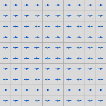
To incorporate only wind direction into your output accumulative surface, you can encode wind direction azimuths (clockwise 0-360 from north; both 0 and 360 are treated as north) in the input horizontal raster. In the image below, a 10 by 10 horizontal raster is shown. It has a constant cell value of 90 and represents wind blowing to the east with some uniform speed over the study area.
Do not use wind speed as the friction in a cost surface, because in a cost surface, the cost is the same regardless of the direction you travel through a cell. A cost friction surface isn't necessary at all.
You can make the cost of motion vary based on the direction of the wind, but you cannot vary the cost of motion for both the direction and the speed of the wind.
Travel from source
In this scenario, the following movement assumptions apply:
- You are sitting on the single source point (the selected cyan point in the center of the raster in the image below).
- It is easiest to move with the wind and impossible to move either against it or at right angles to it.
- You want to calculate accumulated cost from the source cell to every other cell in the study area.
For this scenario, the Horizontal factor parameter is set to Forward. The Travel direction parameter is set to Travel from source. The result is shown below. The output accumulative distance raster is only defined in areas that can be reached travelling with (or somewhat with) the wind.
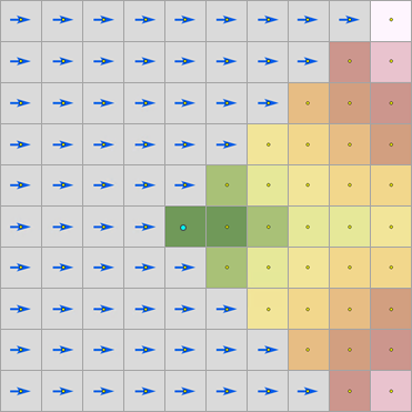
In the image above, the single source is the selected point in the center and you want to know how expensive it is to reach other cells in the study area. The accumulated cost surface shows that you are only allowed to move with the wind, and it is easiest to move directly east.
Zoom in on the single source cell and its eight neighbors to see how Distance Accumulation turns wind direction into travel cost (also known as a weight).
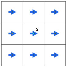
From that source, you can move in eight directions to reach a neighbor cell and you need to determine what the step cost for that move is. Each choice makes a different angle relative to each cell's wind direction.
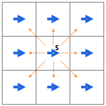
In this case, the only thing that affects the step cost is wind direction. Each step direction makes an angle with the preferred moving direction, which in this case is the wind direction. This angle must be calculated for each neighboring cell. The angle is the horizontal relative moving angle (HRMA) because it is the direction of motion relative to an azimuth value stored in the horizontal raster.
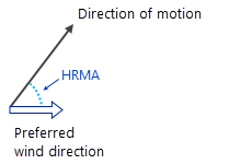
Once the HRMA is identified, a horizontal factor function is applied that turns the HRMA into a weight. In this example, the horizontal factor Forward function is used. For additional information, see Adjust the encountered distance using a horizontal factor.
The HRMA and horizontal factor function are evaluated twice for each of the steps: once for the wind direction at the source cell (from the source center to the edge of the cell) and once for the direction at the neighbor cell (from the edge of the source cell to the center of the neighbor cell). The calculations simulate moving out of the source cell and moving into the neighboring cell. The two results are averaged to get the horizontal weight to use when calculating the cost of a step into the neighbor cell.
Travel to source
In this scenario, the single source point represents a location that you want to reach from other points in the study area. All inputs to Distance Accumulation remain the same, except you choose Travel to source for the Travel direction parameter. The image below shows the result, which is different than the result of the previous scenario.
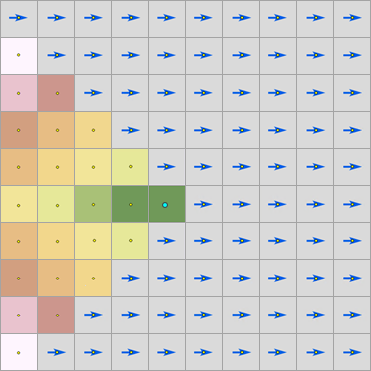
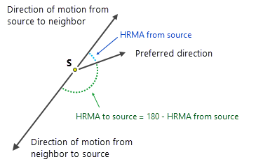
With Travel from source, the accumulative cost surface is grown outward starting from the source and visiting all other cells. With Travel to source, the calculation of the HRMA is different, so the output of the horizontal factor function applied to that HRMA is also different. The HRMA is the geometric supplement of the HRMA calculated in the Travel from source scenario, as shown below.
The Distance Accumulation tool can adjust the cost of motion through a cell based on the easiest direction to move through the cell. This calculation can produce different results depending on if you want to move from a source to other cells, or from other cells to the source.
The logic between Travel Direction and the horizontal factor can be applied to Travel Direction and the vertical factor. However, instead of accounting for horizontal influences, the vertical factor determines the cost to overcome the changes in elevations (slopes) between the cells.