How Cut Fill works—ArcGIS AllSource

A cut-and-fill operation is a procedure in which the elevation of a landform surface is modified by the removal or addition of surface material.

The Cut Fill tool summarizes the areas and volumes of change from a cut-and-fill operation. By taking surfaces of a given location at two different time periods, it identifies regions of surface material removal, surface material addition, and areas where the surface has not changed.

Applications

With the Cut Fill tool, you can do the following:

Identify regions of sediment erosion and deposition in a river valley.
Calculate the volumes and areas of surface material to be removed and areas to be filled to level a site for building construction.
Identify areas that become frequently inundated with surface material during a mudslide in a study to locate safe areas of stable land for building homes.

Display

When the Cut Fill tool is run, by default, a specialized renderer is applied to it that highlights the locations of cut and of fill. The determinant is the attribute table of the output raster and considers positive volume to be where material was cut (removed) and negative volume where material was filled (added).

See the illustration in the tool documentation for an example.

Using Cut Fill for river morphology

Using river morphology as an example to track the amount and location of erosion and deposition in a river valley, a series of cross sections need to be taken through the valley and surveyed on a regular basis to identify regions of sediment erosion and deposition.

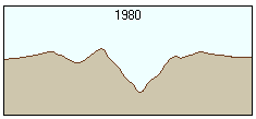
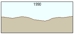
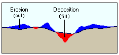
The following graphics show a side profile of one of the cross-sections in the surface that has experienced changes where material has been removed from some areas and added to others.

The first graphic shows the surface in its original state:

Before surface profile

The second graphic shows the surface after a period of time where erosional and depositional forces have acted on it:

After surface profile

The third graphic shows how the Cut Fill tool identifies the areas where material has been removed (cut) and where it has been gained (filled):

Calculations

The output raster retains several properties of the change in its attribute table.

Edge-connected areas identified

First, from the upper-right corner, a sequential value is given to each unique edge-connected area of cut, fill, or no change.

Different types of connectivity are demonstrated in the following graphic:

Volume calculation

For each of the cut/fill regions, the volume is calculated. For a single cell, the formula for the volume is:

  Vol = (cell_area) * ΔZ

where:
```
  ΔZ = Z_Before - Z_After
```

For example, a particular cell has an initial z-value of 235 and a cell size of 10 meters. If the location is excavated by 3 metres, the volume will be:

  Vol = (10m * 10m) * (235m - 232m)
      = 100m² * 3m
      = 300m³

Note:

From the formula, in areas where material has been cut, the volume will be positive (larger value - smaller value > 0). When material was added, the volume will be negative (smaller value - larger value < 0).

Area calculation

For each of the cut/fill regions, the area is also calculated. This is simply the number of cells in the region (Count) multiplied by the cell size of the raster.

Attribute table

An example of the attribute table for the output raster is the following:

ObjectID   Value   Count           Volume        Area
       0       1   55819            0.000   258107056
       1       2     707   -137415060.250     3269168
       2       3      65   -114913516.625      300560
       3       4     810   1235057106.000     3745440

Positive values for volume indicate areas that have had material cut (removed), and negative volume values are for areas that have had material filled (added).