ArcGIS AllSource includes tools that improve and adjust the display of a raster such as providing faster drawing methods and enhancements, and retaining calculated raster dataset statistics. For example, you can change the brightness and contrast of a raster and display the raster transparently over other layers. You can also use geoprocessing tools to permanently improve the display of raster data.
Faster drawing methods
Drawing speeds for raster data is important. This section provides some considerations to help drawing performance, such as pyramids, overviews, footprint wireframe, tile size, and compression.
Pyramids and overviews
The best way to improve and reduce the time it takes to display a large raster dataset is by creating raster pyramids. Pyramids are copies of the original raster dataset that have been successively resampled in decreasing levels of resolution, created as an .ovr file, with the same file name as the raster dataset. Some older pyramids may use the .rrd extension. ArcGIS AllSource uses the appropriate level of resolution to quickly draw the entire dataset. Without pyramids, the entire dataset must be read from disk and resampled to a smaller size for display.
For mosaic datasets, you can build pyramids for each raster dataset, and you can use the Build Overviews tool. Mosaic dataset overviews are similar to raster dataset pyramids; they are lower-resolution images created to increase display speed and reduce CPU usage. However, they differ in that you can control many of the parameters used to create them. You can create overviews to cover only a specific area or at specific resolutions. Overview allow you to view all the rasters contained in the entire mosaic dataset, not only for each raster item.
Footprint wireframe
When you add a mosaic dataset to a map, it is added as a mosaic layer that appears in the Contents pane as a special group layer with a minimum of three layers: Boundary, Footprint, and Image. You can uncheck the Image layer and check the Footprint or Boundary layer to see either the extent of each raster or the extent of the mosaic dataset.
Tile size
Note:
This functionality is only available with (tiled) .tiff files and geodatabases.
The tile size controls the number of pixels, specified in rows and columns, stored in each tile (or block). Each tile is stored as a binary large object (BLOB). By default, the tile size is 128 by 128 pixels, but you can change the value. Changing the tile size does not necessarily improve performance; for an enterprise geodatabase, changing the default can decrease performance.
Raster compression
Compressed data must be decompressed to be drawn on the screen; compressed data generally displays slower than uncompressed data. The amount of time decompression takes is often related to the compression ratio. The more highly compressed the raster, the longer it takes to decompress. There are many types of compression methods available for raster datasets.
Raster data appearance
Raster data appearance can be altered to help render the data for your project needs. This section provides a few techniques to help visualize data, as needed.
Contrast stretch
If the raster data represents continuous data, you can apply a contrast stretch to it based on the statistics of the raster dataset. A stretch increases the visual contrast of the raster display. For example, you can apply a stretch when the raster display appears dark or has little contrast. In these cases, images may not contain the entire range of values your computer can display, so you can stretch the image's values to use this range by applying a contrast stretch. This may result in a crisper image, and some features may become easier to distinguish.
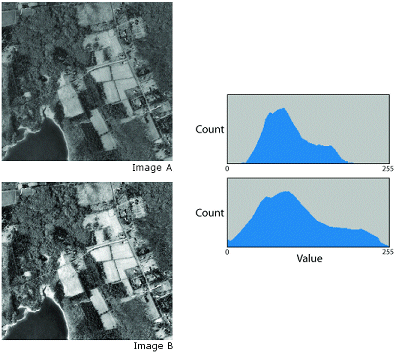
An example of a contrast stretch is shown below. Histogram A represents the pixel values in Image A. By stretching the values (shown in histogram B) across the entire range, you can alter and visually enhance the appearance of the image (Image B).
Different stretches produce different results in the raster display. You can experiment to find the best stretch for a particular raster dataset.
Standard stretches can be used with either the RGB Composite or Stretched renderer. The standard stretches are None, Minimum–Maximum, Percent Clip, Standard Deviation, Histogram Equalize, Custom, and Esri.
The minimum–maximum stretch spreads out tightly grouped values. A two-standard deviation stretch is often used to brighten raster datasets that normally appear dark. A percent clip stretch removes the outliers at the low and high ends of the histogram tails. The histogram equalize stretch spreads out the values across the histogram equally. The custom stretch uses the values from your interactive histogram manipulation. The Esri stretch requires that the raster dataset statistics (and its histogram) be computed or estimated; this method provides a good overall stretch with imagery by preventing pixel values from being stretched to the extremes.
Depending on the stretch method used, you can either examine or modify the histogram to see basic statistics (such as minimum, maximum, mean, and standard deviation) about the data. You can interactively adjust the histograms tails using the Histogram button  for the Minimum–Maximum, Percent Clip, and Standard Deviation stretches. The Custom stretch allows you to manipulate the histogram in a piecewise manner. For more information about viewing and adjusting a histogram, see Histogram stretching.
If you have stretched the entire histogram of your raster dataset and it still isn't being displayed with enough contrast, you can use dynamic range adjustment (DRA) to stretch the pixels within the display's extent. This option allows only the statistics from the pixels within the display extent, rather than the entire raster dataset, to be used to calculate the contrast stretch. Since a smaller number of pixel values exist in the display extent, a smaller range of pixel values will most likely be used, which allows a greater contrast stretch. Each time the display extent (or location) changes, the raster dataset can be displayed differently because the contrast stretch calculated for the pixel values in the display may change. To apply a specific set of statistics to a certain extent, use the Custom Statistics option.
Gamma
You can also apply a gamma stretch to raster data. When preparing raster data for computer display, the gamma refers to the degree of contrast between the mid-level gray values of a raster dataset. Gamma does not affect the lowest or highest values in a raster dataset, only the middle values. By applying a gamma correction, you can control the overall brightness of a raster dataset. Gamma values less than one decrease the contrast in the darker areas and increase the contrast in the lighter areas. This darkens the image without saturating the dark or light areas of the image and brings out details in lighter features. Conversely, gamma values greater than one increase the contrast in darker areas, such as shadows from buildings. Gamma values greater than one can also bring out details in lower elevation areas when working with elevation data. Additionally, gamma changes not only the brightness but also the ratios of red to green to blue.
In the example below, the effect of adjusting the gamma values used to display a raster dataset is shown. Each of the values was added to the red, green, and blue bands. By applying different values to each band, you can adjust the degree of red, green, and blue displayed in the color composite image.

Brightness, contrast, and transparency
You can interactively adjust the brightness  , contrast
  , or gamma
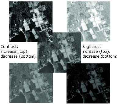
  , which are on the Raster Layer, Mosaic Layer, or Image Service Layer tabs. These enhancements are applied to the rendered screen display, not to the original raster dataset values. Brightness increases the overall lightness of the image—for example, making dark colors lighter and light colors whiter—while contrast adjusts the difference between the darkest and lightest colors. The following is an example of adjustments made to the brightness and contrast of an image:
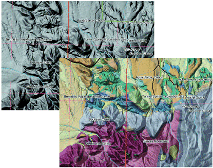
The transparency tool  allows you to see data layers under the raster layer. In the example below, the top image does not use transparency, and the hillshade obscures the underlying land-use layer. With transparency enabled (the bottom image), the underlying symbology appears through the hillshade, producing a three-dimensional effect.
Display resampling
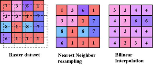
Resampling a raster dataset alters the way it is displayed. Resampling is the process of interpolating new pixel values while transforming the raster dataset when it undergoes a geoprocessing function or when it changes coordinate space. The four resampling techniques are nearest neighbor, bilinear interpolation, cubic convolution, and majority.
For discrete raster datasets, such as those found in classified imagery including land-use maps or soil maps, the nearest neighbor and majority resampling algorithms are most appropriate. The nearest neighbor technique assigns the closest pixel value to the pixel. The majority technique assigns the most popular value in the filter window, providing a smoother look.
For continuous raster datasets—such as a satellite image, an elevation model, or an aerial image—bilinear interpolation or cubic convolution is more appropriate. The bilinear interpolation technique creates a smooth-looking result. The cubic convolution technique creates a sharper-looking result but takes longer to process. The exception is when preserving the radiometry of an image for accurate multispectral analysis; in this case, nearest neighbor is the most appropriate technique.
The diagram below shows an example of display resampling. The first image shows the original raster and the new position of the raster (outline of the raster). The center image shows how the nearest neighbor resampling technique resamples the data. The last image shows how bilinear interpolation resamples the raster.
Background display
You may have homogeneous areas in a raster dataset that you do not want to display. These can include borders, backgrounds, or data that is considered to have no valid values. These can be expressed as NoData values, or they may have real values.
Backgrounds and outlines are sometimes the result of reprojecting the raster dataset. If the raster data has a background, border, or other NoData values, you can choose not to display them, or choose to display them as a particular color.
All renderers allow you to set the NoData value to a color or no color, while the Stretched and RGB renderers allow you to identify a specific background value and display color or no color.
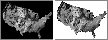
The images below show a NoData area with a black background and the same area using no color.
