Available with Spatial Analyst license.
Available with 3D Analyst license.
The tool uses a global polynomial interpolation that fits a smooth surface defined by a mathematical function (a polynomial) to the input sample points. The trend surface changes gradually and captures coarse-scale patterns in the data.
Conceptual background
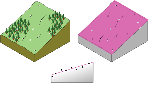
Conceptually, trend interpolation is like taking a piece of paper and fitting it between raised points (raised to the height of value). This is demonstrated in the diagram below for a set of sample points of elevation taken on a gently sloping hill. The piece of paper is magenta.

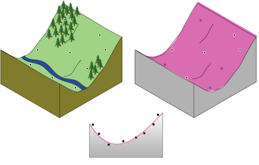
A flat piece of paper will not accurately capture a landscape containing a valley. However, if you bend the piece of paper once, you get a better fit. Adding a term to the mathematical formula produces a similar result, a bend in the plane. A flat plane (no bend in the piece of paper) is a first-order polynomial (linear). Allowing one bend is a second-order polynomial (quadratic), two bends a third-order (cubic), and so forth. A maximum of 12 bends (twelfth order) are allowed with this tool. The following image conceptually demonstrates a second-order polynomial fitted to a valley.

Rarely will the piece of paper pass through the actual measured points, thus making trend interpolation an inexact interpolator. Some points will be above the piece of paper, and others will be below. However, if you add up how much higher each point is above the piece of paper and add up how much lower each point is below the piece of paper, the two sums should be similar. The surface, given in magenta, is obtained by using a least-squares regression fit. The resulting surface minimizes the squared differences among the raised values and the sheet of paper.
The lower the root mean square (RMS) error, the more closely the interpolated surface represents the input points. The most common orders of polynomials are one through three. Trend surface interpolation creates smooth surfaces.
When to use trend interpolation
Trend interpolation results in a smooth surface that represents gradual trends in the surface over the area of interest. This type of interpolation can be used for:
- Fitting a surface to the sample points when the surface varies gradually from region to region over the area of interest—for example, pollution over an industrial area.
- Examining or removing the effects of long-range or global trends. In such circumstances, the technique is often referred to as trend surface analysis.
Trend interpolation creates a gradually varying surface using low-order polynomials that describe a physical process—for example, pollution and wind direction. However, the more complex the polynomial, the more difficult it is to ascribe physical meaning to it. Furthermore, the calculated surfaces are highly susceptible to outliers (extremely high and low values), especially at the edges.
Types of trend interpolation
There are two basic types of Trend interpolation: Linear and Logistic.
Linear trend
The Linear trend surface interpolator creates a floating-point raster. It uses a polynomial regression to fit a least-squares surface to the input points. This method allows you to control the order of the polynomial used to fit the surface. To understand this method, consider a first-order polynomial. A first-order linear trend surface interpolation performs a least-squares fit of a plane to the set of input points.
Trend surface interpolation creates smooth surfaces. The surface generated seldom passes through the original data points, since it performs a best fit for the entire surface. When a polynomial order higher than one is used, the interpolator may generate a raster whose minimum and maximum exceed the minimum and maximum of the input file of the input feature data.
Logistic trend
The Logistic option for generating a trend surface is appropriate for prediction of the presence or absence of certain phenomena (in the form of probability) for a given set of locations (x,y) in space. The z-value is a categorized random variable with only two possible outcomes—for example, the existence of an endangered species or the lack of existence of that species. These two z-values can be coded as one and zero, respectively. This option creates a continuous probability grid with cell values between one and zero.
A maximum likelihood estimation is used to calculate the nonlinear probability surface model without first converting the model into linear form.
Output RMS file
The RMS error file contains the root mean square error of the interpolation by comparing the value of the locations in the input dataset against the value of those same locations in the interpolated raster surface.
The RMS error value can be used to determine the best value to use for the {order} parameter of the interpolation by changing the order value until you get the lowest RMS error. The Chi-square value is also reported.
Example
An example of the output RMS file from a run of the Trend tool with the Polynomial order set to 3 is:
coef #          coef
------ ----------------
     0 -1192066.7888371
     1 -1.78479492586755
     2 -0.195982103615487
     3 -8.87072249743903e-1
     4 -2.0538267625596e-1
     5 -3.85610088343239e-1
     6 -1.46420255709888e-2
     7 -5.31539027745154e-2
     8 -2.59261094879031e-3
     9 9.71651459136166e-4
------ ----------------
RMS Error  = 296.957857221845
Chi-Square  = 17019506.0103975
The predicted value at any location in the output raster for this third-order trend can be determined by summing up the values that result from a series of equations. For these equations, x = the longitude of the location, y = the latitude, and the cn term is the coefficient value from the preceding table. The equations for this third-order interpolation are:
Prediction(x,y) = c0 +
                  x·c1 + y·c2 +
                  x2·c3 + x·y·c4 + y2·c5 +
                  x3·c6 + x2·y·c7 + x·y2·c8 + y3·c9
Essentially, coefficient 0 is always the intercept. From there, iterate through the first-order terms starting with the highest x and ending with no xs. Move to the second-order terms and iterate down the xs again, and similarly for the third-order terms.
Note:
These equations follow a similar pattern as the order increases. For example, if the fourth order was specified, there would be five more values specified in the RMS table (coefficients 10, 11, 12, 13 and 14) and commensurately more equations that utilize them.