Object Detection

Available with Image Analyst license.

The following methods and concepts are key to understanding and performing object detection in ArcGIS AllSource.

Single Shot Detector (SSD)

Single Shot Detector (SSD) takes a single pass over the image to detect multiple objects. SSD is considered one of the faster object detection model types with fairly high accuracy.

SSD has two components: a backbone model and SSD head. The backbone model is a pretrained image classification network as a feature extractor. This is typically a network such as ResNet trained on Imagenet from which the final fully connected classification layer has been removed. The SSD head is just one or more convolutional layers added to this backbone, and the outputs are interpreted as the bounding boxes and classes of objects in the spatial location of the final layers' activations.

Grid cell

Instead of using a sliding window, SSD divides the image using a grid, and each grid cell is responsible for detecting objects in that region of the image. Detecting objects means predicting the class and location of an object within that region. If no object is present, it is considered the background class and the location is ignored. For instance, you can use a 4 by 4 grid in the example below. Each grid cell can output the position and shape of the object it contains.

An example of a 4 by 4 grid is shown.

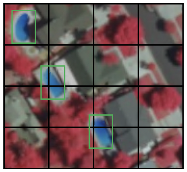
If there are multiple objects in one grid cell or you need to detect multiple objects of different shapes, the anchor box will be used.

Anchor box

Each grid cell in SSD can be assigned multiple anchor (or prior) boxes. These anchor boxes are predefined, and each one is responsible for a size and shape within a grid cell. For example, the swimming pool in the image below corresponds to the taller anchor box while the building corresponds to the wider box.

An example of two anchor boxes is shown.

The legend of the two anchor boxes is shown.

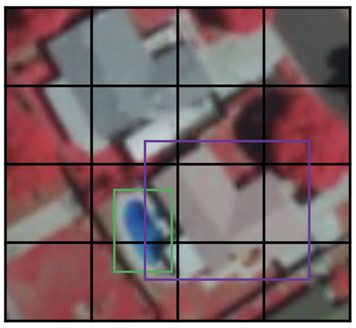
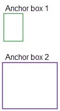
SSD uses a matching phase while training to match the appropriate anchor box with the bounding boxes of each ground truth object within an image. Essentially, the anchor box with the highest degree of overlap with an object is responsible for predicting that object’s class and its location. This property is used for training the network and for predicting the detected objects and their locations once the network has been trained. In practice, each anchor box is specified by an aspect ratio and a zoom level.

Aspect ratio

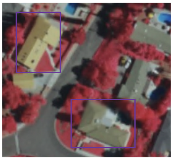
Not all objects are square in shape. Some are longer, and some are wider, by varying degrees. The SSD architecture allows predefined aspect ratios of the anchor boxes to account for this. You can use the ratios parameter to specify the different aspect ratios of the anchor boxes associated with each grid cell at each zoom or scale level.

The bounding box of building 1 is higher, while the bounding box for building 2 is wider.

Zoom level

It is not necessary for the anchor boxes to have the same size as the grid cell. You may want to find smaller or larger objects within a grid cell. The zooms parameter is used to specify how much you need to scale the anchor boxes up or down with respect to each grid cell. As in the anchor box example, the size of building is generally larger than swimming pool.

RetinaNet

RetinaNet is a one-stage object detection model that works well with dense and small-scale objects. For this reason, it has become a popular object detection model to use with aerial and satellite imagery.

Architecture

There are four major components of a RetinaNet model architecture¹:

• Bottom-up Pathway—The backbone network of ResNet, which calculates the feature maps at different scales, irrespective of the input image size or the backbone.
• Top-down pathway and Lateral connections—The top down pathway upsamples the spatially coarser feature maps from higher pyramid levels, and the lateral connections merge the top-down layers and the bottom-up layers with the same spatial size.
• Classification subnetwork—Predicts the probability of an object being present at each spatial location for each anchor box and object class.
• Regression subnetwork— Regresses the offset for the bounding boxes from the anchor boxes for each ground-truth object.

Focal Loss

Focal Loss (FL) is an enhancement over Cross-Entropy Loss (CE) and is introduced to handle the class imbalance problem with single-stage object detection models. Single Stage models suffer from an extreme foreground-background class imbalance problem due to dense sampling of anchor boxes (possible object locations¹). In RetinaNet, each pyramid layer can have thousands of anchor boxes. Only a few are assigned to a ground-truth object while the vast majority will be background class. These easy examples (detections with high probabilities) result in small loss values but can collectively overwhelm the model. FL reduces the loss contribution from easy examples and increases the importance of correcting misclassified examples.

Scales

The scale of anchor boxes. The default is set to [2, 2.3, 2.6] which works well with most of the objects in any dataset. You can change the scales according to the size of objects in your dataset.

Aspect ratio

The aspect ratio of anchor boxes. The default is set to [0.5, 1, 2] which means the anchor boxes will be of aspect ratios 1:2, 1:1, 2:1. You can modify the ratios according to the shape of the objects of interest.

YOLOv3

YOLO (You Only Look Once ) v3 uses Darknet-53 as its backbone. This is in contrast to the use of popular ResNet family of backbones by other models, such as SSD and RetinaNet. Darknet-53 is a deeper version of Darknet-19, which was used in YOLOv2, a prior version. As the name suggests, this backbone architecture has 53 convolutional layers. Adapting the ResNet style residual layers has improved its accuracy while maintaining the speed advantage. This feature extractor performs better than ResNet101 and similar to ResNet152 while being about 1.5 times and 2 times faster, respectively².

YOLOv3 has incremental improvements over its prior versions². It uses upsampling and concatenation of feature layers with earlier feature layers that preserve fine-grained features. Another improvement is using three scales for detection. This has made the model good at detecting objects of varying scales in an image. There are other improvements in anchor box selections, loss function, and so on. For a detailed analysis of the YOLOv3 architecture, refer to What's new in YOLO v3? .

Faster R-CNN

Before Faster R-CNN (Region-based Convolutional Neural Network), models were using various algorithms for region proposal that were being computed on the CPU and creating a bottleneck. Faster R-CNN has improved the object detection architecture by replacing the selection search algorithm in Fast R-CNN with a convolutional network called the Region Proposal Network (RPN). The rest of the model architecture remains the same as Fast R-CNN; the image is fed to a CNN to produce a feature map from which features for regions proposed by the RPN are selected and resized by a pooling layer and fed to an FC layer with two heads—a softmax classifier and a bounding box regressor. This design increased the speed of detection and brought it closer to real time³.

Architecture for Faster R-CNN is shown³.

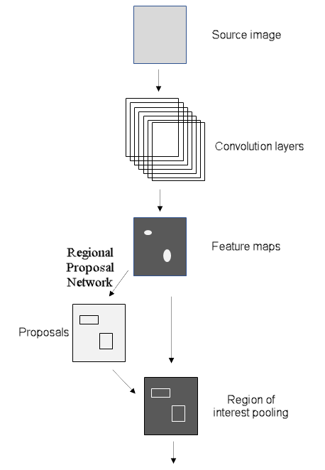
Regional Proposal Network

Region Proposal Network (RPC) inputs an image and returns regions of interest that contain objects, much like other region proposal algorithms. RPN also returns an object score, which measures the likelihood that the region will have an object, instead of a background³. In Faster R-CNN, the RPN and the detect network shares the same backbone; the last shared layer of the backbone provides a feature map of the image that is used by the RPN to propose regions.

Using a sliding window approach, a small network is overlaid onto the feature map. At each spatial window, there are multiple anchor boxes that are of predetermined scales and aspect ratios. This enables the model to detect objects of a wide range of scales and aspect ratios in the same image. Usually the anchor boxes are created at three different scales and three different aspect ratios, resulting in nine anchor boxes at each spatial location that denotes the maximum region proposals at that spatial location. The small network then feeds into fully connected layers with two heads—one for the object score and the other for the bounding box coordinates of the region proposals. Note that these layers, though similar to the last few layers of the Fast R-CNN object detector, are not the same nor do they share the weights. The RPN classifies the regions in a class agnostic manner as it is tasked with only finding the regions that contain the objects. For more information about RPN, see Faster R-CNN for object detection .

Mask R-CNN

Mask R-CNN is a model for instance segmentation. It was developed on the Faster R-CNN model. The Faster R-CNN model is a region-based convolutional neural networks⁴ that returns bounding boxes for each object and its class label with a confidence score.

Faster R-CNN predicts object class and bounding boxes, but Mask R-CNN is an extension of Faster R-CNN with additional branches for predicting segmentation masks on each region of interest (RoI). In the second stage of Faster R-CNN, the RoI pool is replaced by RoIAlign, which helps to preserve spatial information that gets misaligned in case of RoI pool. RoIAlign uses binary interpolation to create a feature map that is of fixed size, for example 7 by 7. The output from the RoIAlign layer is then fed into Mask head, which consists of two convolution layers. It generates mask for each RoI, thus segmenting an image in a pixel-to-pixel manner. To avoid oversmoothing the boundaries that are not precise, for objects with irregular boundaries, the model has been enhanced to include a point-based rendering neural network module called PointRend.

Instance Segmentation

Instance Segmentation integrates an object detection task—where the goal is to detect an object and its bounding box prediction in an image—and semantic segmentation task, which classifies each pixel into predefined categories. Thus, you can detect objects in an image while precisely segmenting a mask for each object instance.

Instance segmentation allows you to solve many problems, such as the following:

• Damage detection, where it is important to know extent of damage.
• Self-driving cars, where it is important to know the position of each car in the scene.
• Generating building footprints for each individual building—a common problem in GIS.

References

[1] Tsung-Yi Lin, Priya Goyal, Ross Girshick, Kaiming He, and Piotr Dollár. Focal Loss for Dense Object Detection, http://arxiv.org/abs/1708.02002 arXiv:1708.02002, (2017).

[2] Joseph Redmon, Ali Farhadi. YOLOv3: An Incremental Improvement, https://arxiv.org/abs/1804.02767 arXiv:1804.02767, (2018).

[3] Shaoqing Ren, Kaiming He, Ross Girshick, and Jian Sun. Faster R-CNN: Towards Real-Time Object Detection with Region Proposal Networks, http://arxiv.org/abs/1506.01497 arXiv:1506.01497, (2015).

[4] Shaoqing Ren, Kaiming He, Ross Girshick, and Jian Sun. Faster R-CNN: Towards Real-Time Object Detection with Region Proposal Networks, http://arxiv.org/abs/1506.01497 arXiv:1506.01497, (2015).