An index is a number that measures a subject of interest, often something that is difficult to directly measure or define, such as social vulnerability or business innovation. The Calculate Composite Index tool creates an index by combining multiple variables into a single variable. The tool follows a three-step workflow to preprocess the variables, combine the variables, and postprocess the index.
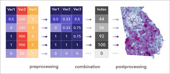
The proper building of an index relies on the thorough consideration of its purpose during design and transparency of the process during communication. The Calculate Composite Index tool guides you through the process of building an appropriate index and helps you visualize and understand the results.
Learn more about best practices for creating composite indices in ArcGIS
Potential applications
The following are potential applications of the Calculate Composite Index tool:
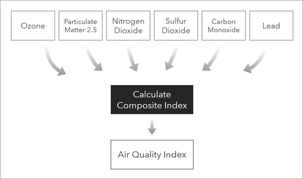
- An environmental protection department wants to create an air quality index to inform public policy and the public about pollution. They collect data from monitoring stations corresponding to criteria pollutants. An analyst can run the Calculate Composite Index tool to combine the individual pollutant indicators into a single air quality index.
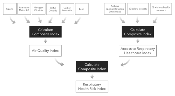
- A public health department wants to create a respiratory health risk index to highlight environmental injustices. To do this, the analyst can run the Calculate Composite Index tool multiple times to create an index with multiple subindices, in which the first run of the tool creates subindices for different domains and the last run of the tool creates the final index.
- A jurisdiction wants to apply for an infrastructure grant, and to qualify they need to prove that resources will go to underserved communities. They can create an index that combines infrastructure and demographic variables to identify the most underserved areas.
How variables are preprocessed
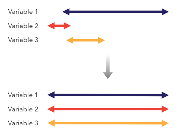
To create an appropriate index, variables must be in a compatible scale. To achieve this, preprocessing options are offered in the tool that bring different input variables to a common measurement scale so they can be appropriately combined. The tool also optionally reverses variables so that the meaning of high values in each variable align with each other.
Note:
Use the Transform Field tool to transform variables.
Preprocess variables to reverse direction
Consider the meaning of low and high values in each variable and ensure they are consistent with each other. For example, in a social vulnerability index, locations with lower median incomes are more vulnerable, but locations with low percentages of people without insurance are less vulnerable; the direction of these variables are opposed in the context of the purpose of the index.
As you enter each variable into the tool, consider whether the variable should be reversed; in which case, check the Reverse Direction check box to reverse the direction of the variable.
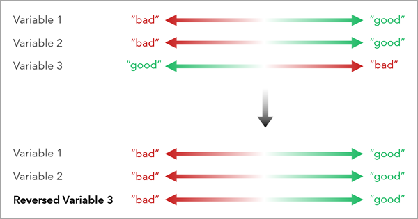
The reverse of the variable is calculated by multiplying each value by -1 and scaling the field between the original range of the variable.
Preprocess variables to use the same scale
Use the Method to Scale Input Variables parameter to select a common scale method. The selected method will be applied to all variables and the resulting fields are provided in the output. The following options are available:
Minimum-maximum—This method scales the variables between 0 and 1 using the minimum and maximum values of each variable. This method is the simplest, as it preserves the distribution of the input variables and scales to a 0 to 1 scale that is easy to interpret.
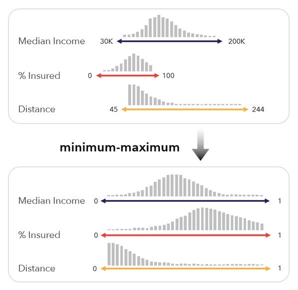
This method applies the following formula:

Since this method preserves the variable distribution, it can be affected by skewed distributions and outliers. For example, if there is a single outlier with a very high value, the outlier will receive a value of 1, but the rest of the values will be similar and closer to zero. As a consequence of the reduced variation in the preprocessed variable, this variable may have less influence on the resulting index.
This method also depends on the minimum and maximum values in the input data, making it less appropriate for index comparisons across multiple time periods, when a variable's minimum and maximum values may change with each time step.
Minimum-maximum (custom data ranges)—This method scales the variables between 0 and 1 using the possible minimum and possible maximum values for each variable. This method is useful when the possible minimum and maximum do not exist in the range of the variable, or you want to create an index that must remain comparable as additional data is collected.
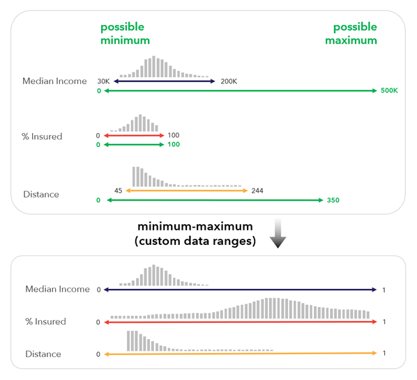
This method applies the following formula:

There are multiple use cases for setting a possible minimum and possible maximum:
- When the index will be compared across time, and the current data does not represent the range of values that the index could have in other time periods.
- When there is a reference statistic, such as a broader study area's minimum and maximum. For example, an index with a study area set in France may use a minimum and maximum based on all countries in Europe.
- When there is an aspirational benchmark, such as the aspirational life expectancy in a human development index. While the data itself may not have the aspired life expectancy, the benchmark is still used to set context for the index.
- When there is a priori knowledge of the theoretical minimum and maximum values for variables, such as knowing the absolute temperature ranges on Earth and using daily recordings with a smaller range.
Percentile—This method converts the variables to percentiles between 0 and 1. This method can be useful when the ranks of each variable are more important than their actual values. It is also robust to outliers and skewed distributions, as the variables are transformed to a uniform distribution.
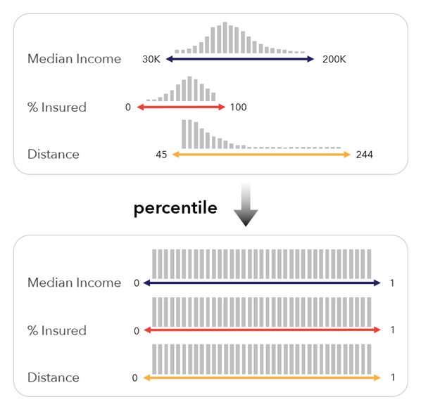
There are various definitions for percentiles. This method uses the following formula:
 ,
,where R is the ordinal rank (using the minimum rank value in the case of ties), N is the number of values, and P is the resulting percentile.
Percentiles denote the position of a value relative to the other values within the variable. For example, while the difference in income between $50,000 and $60,000 may not be substantial, the percentile difference may be large if there are many features with values in between.
Rank—This method ranks the input values, assigning a value of 1 to the lowest value in the variable and incrementing by 1 for each value. This method can be useful when the ranks of each variable are more important than their actual values. The method is also robust to outliers and skewed distributions.
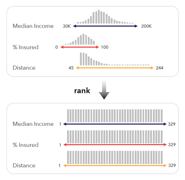
The method uses the rank average method, which resolves ties by assigning the mean rank value to tied observations.
This method is very similar to percentiles, but the range of the values is between 1 and the number of records in the table.
Z-score—This method standardizes each variable using the Z-score formula. This method is useful when each value should be considered with respect to the variable's mean. For example, when you want to know whether the percent of people below the poverty line is higher or lower than the national average, and by how much.
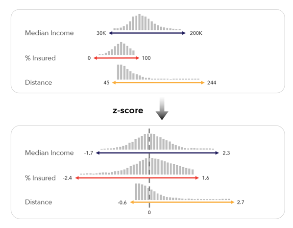
This method uses the following formula:
 ,
,where x' is the z-score, x is the original value, x̄ is the mean (average), and σ is the standard deviation.
Z-scores are expressed in standard deviations, a measure of dispersion in the data. A z-score of 2 means that the feature is two standard deviations greater than the mean, and a z-score of -1 is one standard deviation less than the mean. The method is less susceptible to adverse effects from outliers when compared with the minimum-maximum method. However, it produces negative values, making it incompatible with multiplicative combination methods.
Z-score (custom)—This method standardizes each variable by using the z-score formula with a custom mean and custom standard deviation. This method is useful when creating indices that compare against a reference statistic or compare across time.
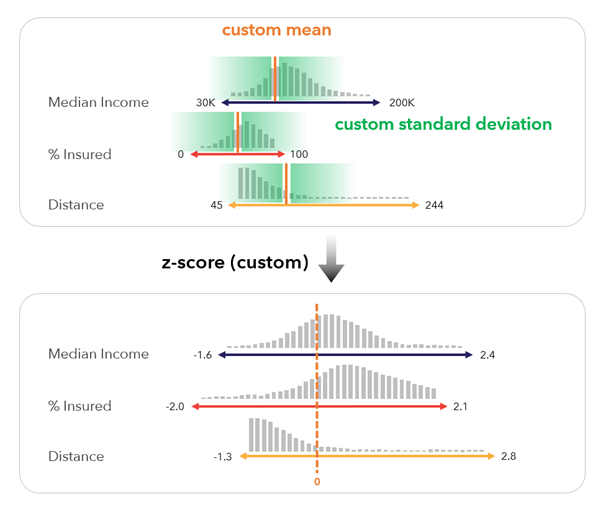
This method uses the following formula:
 ,
,where x' is the standardized value, x is the original value, x̄c is the custom mean, and σc is the custom standard deviation.
Use the Custom Standardization parameter to set the reference mean and standard deviation.
For example, to create an annual development index that will be updated for the next 10 years using the first year as the comparison point, create an index for the first year using the z-score option which uses the actual mean and standard deviation for each variable. Then use the same mean and standard deviation in the Custom Standardization parameter in subsequent years. This makes the results comparable across all years using the first year's distribution as the comparison.
This method is also useful when comparing values to a theoretical mean that may not equal the data's mean. For example, if the national unemployment rate is 8 percent, but the average unemployment rate in the data is 13 percent, the z-scores can be set in relation to a national average and national standard deviation, and the sample in the data will have more positive values to reflect the unemployment rate being higher than a national average.
Flag by threshold (binary)—This method converts the variable to binary values (0, 1) which indicate whether the value is above or below a specified threshold. This method is useful when it is important to highlight certain values and the variation of the values does not matter.
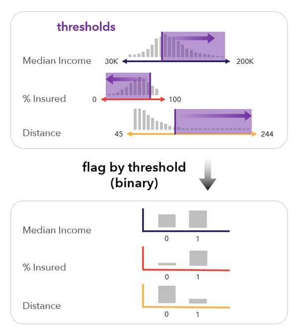
This option activates the Method to Scale for Thresholds parameter, which allows the thresholds to be set in the range of a scaled variable.
There are a variety of use cases for this method:
- Air quality domain experts want to highlight locations that exceed thresholds for human health for multiple air quality variables. They set the Method to Scale for Thresholds parameter variables to raw and specify the thresholds.
- A government agency wants to highlight locations that are highly vulnerable in multiple domains. They set the Method to Scale for Thresholds parameter to percentile and set the threshold to Greater than 0.9 for each variable to highlight the most deprived locations.
- An international organization wants to highlight countries that are consistently below average for human development indicators. They set the Method to Scale for Thresholds parameter to z-score and set the thresholds to Less than 0 to identify locations below the mean.
This method is most useful when combined with the sum combination option to count the number of times a location exceeds the thresholds.
The method is not affected by outliers in the input variables, but the interval level information in each input variable is lost, as each variable is converted to a binary (0, 1) form.
Raw values—Uses the original values of the variable.
This method should only be used if all variables are on a comparable scale. For example, when all variables are a standard unit like percentages or parts per million. This method can also be useful when variable standardization or transformation has already occurred prior to running the tool.
Note:
The selected scaling option is applied to all variables. When you need to apply different scaling options to each variable, use other tools such as Standardize Field or Reclassify Field prior to using this tool.
If a field has any nulls, the tool will not be able to calculate an index for the records. Consider using the Fill Missing Values tool to impute a value, if appropriate, or find supplemental data if not.
How the tool combines variables into an index
Once variables are preprocessed to a common scale, the variables are aggregated to create a single value. The Method to Combine Scaled Variables parameter has the following options:
- Sum
- Mean
- Multiply
- Geometric mean
The Sum and Mean options are considered additive methods, and the Multiply and Geometric mean options are considered multiplicative methods.
Additive methods
The Sum and Mean combination methods are relatively simple to interpret and are commonly used by a variety of indices. The methods are almost identical; they result in distributions with the same shape that only differ in scale, and therefore the resulting index map will look the same. Only the values differ.
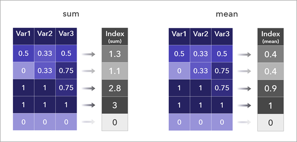
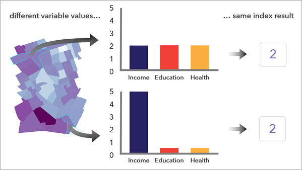
These methods allow high values in one variable to compensate for low values in another variable.
Multiplicative methods
The Multiply and Geometric mean methods require more caution to use, as the resulting index values can be much higher than when using an additive method and the methods do not work well when using negative values.
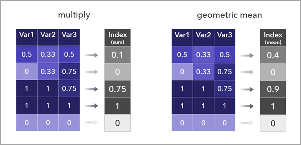
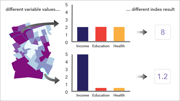
Despite their disadvantages, multiplicative methods have the advantage that they do not allow high values in one variable to compensate for low values in another variable; for an index value to be high, multiple variables must have high values.
Note:
The Preset Method to Scale and Combine Variables parameter provides templates that set the preprocessing and combination methods based on commonly used approaches for creating indices.
Weighting
Variables can be weighted to represent the relative importance of each factor as it contributes to the index. By default, all weights are set to 1, meaning that each variable is equally weighted. However, it may be important to denote differences in the relative contributions of a variable compared to the others. By changing one of the variables to a weight of 2 and keeping the others at 1, you denote that the variable should be considered twice as important as the others in its contribution to the final index.
You may also use weights that add up to 1: for example, if three variables are used, and one should be considered to be twice as important as the other two, you may use weight values of 0.5, 0.25, and 0.25.
In additive methods, weights are applied by multiplying each variable by its respective weight. In multiplicative methods, weights are applied by raising each variable to the power of its respective weight.
Weights have a significant impact on the resulting index. Whether you choose to keep equal weights or alter weights to favor variables, using weights adds subjectivity to the analysis. Additionally, you may unintentionally be weighting due to correlation and differences in variance between your variables. To learn more about the impact of correlation and variance on the index, consult the best practices document for creating composite indices.
How the index is postprocessed
Once variables are preprocessed and combined into the raw index, postprocessing may help make the index more understandable. Options in the Output Settings parameter category allow you to adjust the direction, adjust the scale, and classify the values.
Reverse the index
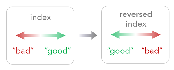
Consider the purpose of the index, and evaluate whether high index values are as intended. Use the Reverse Output Index Values parameter check box to optionally reverse the raw index so that high values become low values and vice-versa.
Note:
Reversing the index values for multiplicative methods should be done with caution, as these results will differ from reversing the input variables.
Scale the index using minimum and maximum values
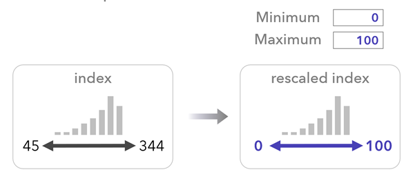
Use the Output Index Minimum and Maximum Values parameter to specify the range of the output index. This option can be useful to use a scale that may be easier to interpret, regardless of the preprocessing and combination methods selected. For example, specify a Minimum value of 0 and a Maximum value of 100 to scale the raw index to this range. The option uses the following formula:
 ,
,
where x is the original value, min(x) is the minimum value found in the index, max(x) is the maximum value found in the index, a is the specified minimum value, b is the specified maximum value, and x' is the scaled value.
Classify the index
In addition to the raw index output, you may optionally classify the output index to help you interrogate the results. The Additional Classified Outputs parameter has four methods that can be used: Equal interval, Quantile, Standard deviation, and Custom, each resulting in an additional field in the output.
The equal intervals method divides the index range into intervals of equal length.

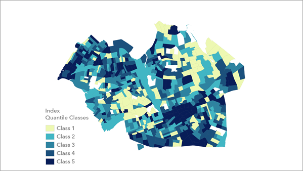
The quantile method divides the values into classes so that each class has the same number of features or rows. This method produces a similar map to the index percentile layer but uses classes, unlike the continuous percentile distribution. Use this option to create a map of quintiles (with five classes), deciles (with 10 classes), or other types of quantiles based on the number of classes.

The standard deviation method classifies the index to show the number of standard deviations each value lies from the mean.

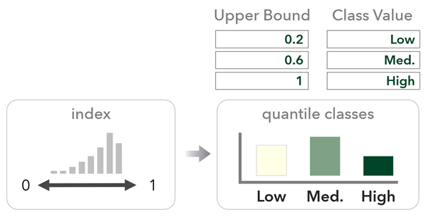
The custom classes method categorizes the continuous index using custom class bounds and custom labels. You can add numeric labels or text labels, such as Low, Medium, and High.
Interpret results
Visualizing and investigating the resulting index is an important step in preparing the index for further use. The tool produces various maps and charts to help you interpret the result.
Output layers
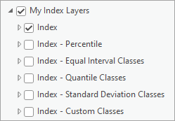
When the Output Features or Table parameter is set to a feature class or shapefile (rather than appending to the input), the tool creates multiple layers that are included in the output group layer:
Tip:
Use the Ctrl and Shift shortcuts to quickly visualize or collapse layers within the group layer.
The index layer displays the distribution of index values after any optional scaling or reversing. The layer provides a continuous choropleth map that can be used to evaluate the index results. You can use the map to evaluate high and low index values, preserving the index distribution and any outliers.
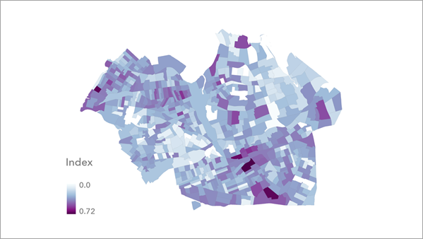
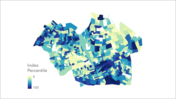
The index percentile layer displays the relative positions (ranks) between index values. The resulting map colors correspond to the ranks of the index values, so they do not preserve the distribution or any sense of actual index differences. Use this method when you want to evaluate how locations relate to each other based on their index rank.
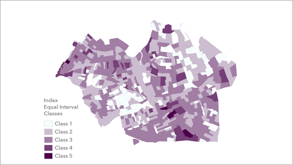
The index equal interval classes layer shows classes based on the index distribution of values, but it groups values together into classes based on equal intervals set by the Output Index Number of Classes parameter. This layer is a classified form of the index layer.
The index quantile layer assigns an equal number of features to each class and is a classified form of the index percentile layer. The number of classes are set by the Output Index Number of Classes parameter.
The index standard deviation classes layer visualizes locations above and below the index mean. The color scheme helps emphasize extremely high and low index values, which can be useful to identify locations that may need further investigation.
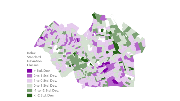
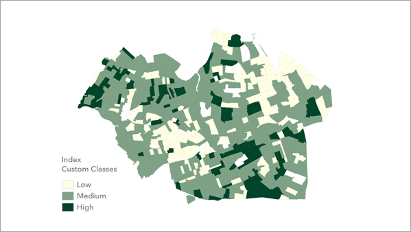
The index custom classes layer displays the specified categories on the map and can be used for many purposes, such as to split a continuous index into uneven categories based on planned interventions. For example, you can name classes Low, Medium, and High.
Output charts
The tool produces charts that can be used to help answer various questions about the index.
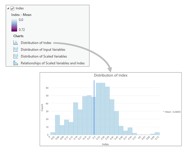
Explore the distribution of the index
The primary index layer in the group layer output contains a histogram of the index distribution. Along with the map, this can help you gain an understanding of the distribution of the results.
Explore the distributions of the input variables
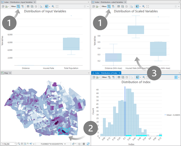
The primary index layer contains two box plots of the input variables: one visualizing the variable distributions prior to scaling and one visualizing variable distributions after scaling. It is often useful to compare these charts side-by-side to evaluate how the selected scaling method changed the input variables. Comparing these charts side-by-side can help evaluate whether the selected scaling method had the intended effect on the distribution of the variables.
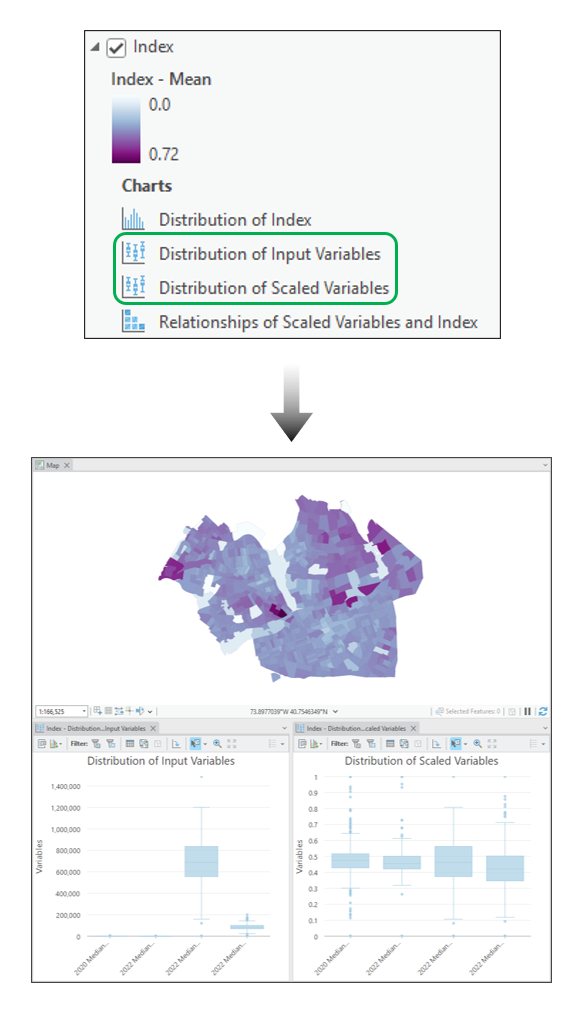
You may also use the box plots to investigate outliers by selecting the outliers on the box plot of input variables and checking their location on the map. You can then view the box plot of preprocessed variables to check if the chosen preprocessing method has remediated the effect of the outlier.
Explore the results of each feature
By opening the map, the histogram, and the two box plots and then activating selection filters on the two box plots, you can select a feature on the map or on the histogram to visualize the distribution of input variable values for the selection. You can also use the map and the extent filters on the box plots to evaluate the variable distribution in different regions of the map.
Explore which variables impact the index
The index layer includes a scatterplot matrix that displays the correlation between the index and each variable used. The variables with high correlation against the index will generally correspond to the variables that contributed most significantly to the index. Consequently, any variables with low correlation with the index may be considered to have less impact on the index. Additionally, consider whether any variables have low internal variation; variables with low variation are less likely to contribute meaningful information to your index.
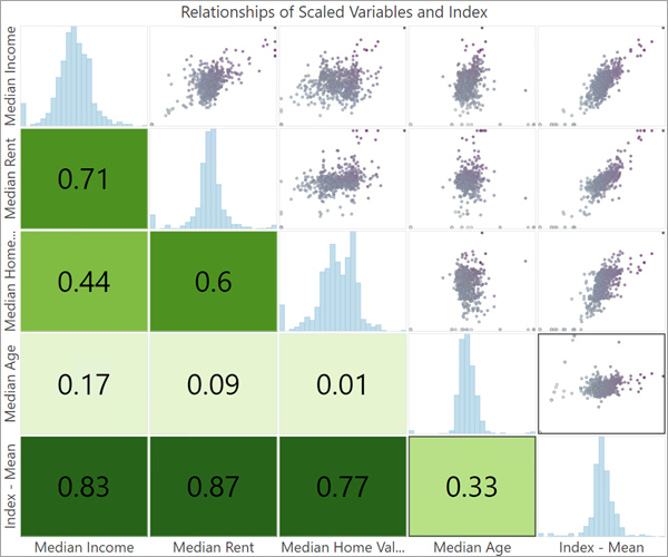
The resulting maps and data visualizations encourage further adjustments and refinement of the index. To learn more about additional considerations when creating and evaluating an index, consult the best practices technical paper.
Additional resources
See the Organisation for Economic Co-operation and Development Handbook on Constructing Composite Indicators: Methodology and User Guide.