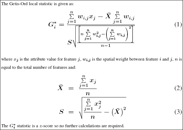
The Hot Spot Analysis tool calculates the Getis-Ord Gi* statistic (pronounced G-i-star) for each feature in a dataset. The resultant z-scores and p-values tell you where features with either high or low values cluster spatially. This tool works by looking at each feature within the context of neighboring features. A feature with a high value is interesting but may not be a statistically significant hot spot. To be a statistically significant hot spot, a feature will have a high value and be surrounded by other features with high values as well. The local sum for a feature and its neighbors is compared proportionally to the sum of all features; when the local sum is very different from the expected local sum, and when that difference is too large to be the result of random chance, a statistically significant z-score results. When the FDR correction is applied, statistical significance is adjusted to account for multiple testing and spatial dependency.
Calculations

Interpretation
The Gi* statistic returned for each feature in the dataset is a z-score. For statistically significant positive z-scores, the larger the z-score is, the more intense the clustering of high values (hot spot). For statistically significant negative z-scores, the smaller the z-score is, the more intense the clustering of low values (cold spot). For more information about determining statistical significance and correcting for multiple testing and spatial dependency, see What is a z-score? What is a p-value?
Output
This tool creates a new Output Feature Class with a z-score, p-value, and confidence level bin (Gi_Bin) for each feature in the Input Feature Class. If there is a selection set applied to the Input Feature Class, only selected features will be analyzed, and only selected features will appear in the Output Feature Class.
When this tool runs in ArcMap, the Output Feature Class is automatically added to the table of contents with default rendering applied to the Gi_Bin field.
Hot spot analysis considerations
There are three things to consider when undertaking any hot spot analysis:
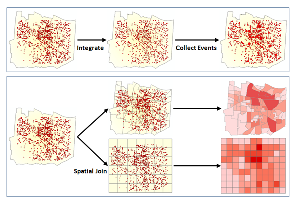
- What is the Analysis Field (Input Field)? The hot spot analysis tool assesses whether high or low values (the number of crimes, accident severity, or dollars spent on sporting goods, for example) cluster spatially. The field containing those values is your Analysis Field. For point incident data, however, you may be more interested in assessing incident intensity than in analyzing the spatial clustering of any particular value associated with the incidents. In that case, you will need to aggregate your incident data prior to analysis. There are several ways to do this:
- If you have polygon features for your study area, you can use the Spatial Join tool to count the number of events in each polygon. The resultant field containing the number of events in each polygon becomes the Input Field for analysis.
- Use the Create Fishnet tool to construct a polygon grid over your point features. Then use the Spatial Join tool to count the number of events falling within each grid polygon. Remove any grid polygons that fall outside your study area. Also, in cases where many of the grid polygons within the study area contain zeros for the number of events, increase the polygon grid size, if appropriate, or remove those zero-count grid polygons prior to analysis.
- Alternatively, if you have a number of coincident points or points within a short distance of one another, you can use Integrate with the Collect Events tool to (1) snap features within a specified distance of each other together, then (2) create a new feature class containing a point at each unique location with an associated count attribute to indicate the number of events/snapped points. Use the resultant ICOUNT field as your Input Field for analysis.
Note:
If you are concerned that your coincident points may be redundant records, the Find Identical tool can help you to locate and remove duplicates.

Strategies for aggregating incident data - Which Conceptualization of Spatial Relationships is appropriate? What Distance Band or Threshold Distance value is best?
The recommended (and default) Conceptualization of Spatial Relationships for the Hot Spot Analysis (Getis-Ord Gi*) tool is Fixed Distance Band. Space-Time Window, Zone of Indifference, Contiguity, K Nearest Neighbor, and Delaunay Triangulation may also work well. For a discussion of best practices and strategies for determining an analysis distance value, see Selecting a Conceptualization of Spatial Relationships and Selecting a Fixed Distance. For more information about space-time hot spot analysis, see Space-Time Analysis.
- What is the question?
This may seem obvious, but how you construct the Input Field for analysis determines the types of questions you can ask. Are you most interested in determining where you have lots of incidents, or where high/low values for a particular attribute cluster spatially? If so, run Hot Spot Analysis on the raw values or raw incident counts. This type of analysis is particularly helpful for resource allocation types of problems. Alternatively (or in addition), you may be interested in locating areas with unexpectedly high values in relation to some other variable. If you are analyzing foreclosures, for example, you probably expect more foreclosures in locations with more homes (said another way, at some level, you expect the number of foreclosures to be a function of the number of houses). If you divide the number of foreclosures by the number of homes, then run the Hot Spot Analysis tool on this ratio, you are no longer asking Where are there lots of foreclosures?; instead, you are asking Where are there unexpectedly high numbers of foreclosures, given the number of homes? By creating a rate or ratio prior to analysis, you can control for certain expected relationships (for example, the number of crimes is a function of population; the number of foreclosures is a function of housing stock) and identify unexpected hot/cold spots.
Best practice guidelines
- Does the Input Feature Class contain at least 30 features? Results aren't reliable with less than 30 features.
- Is the Distance Band or Threshold Distance appropriate? See Selecting a Fixed Distance.
- All features should have at least one neighbor.
- No feature should have all other features as neighbors.
- Especially if the values for the Input Field are skewed, you want features to have about eight neighbors each. The Calculate Distance Band From Neighbor Count tool can be used to find the average distance at which each feature has 8 neighbors.
Potential applications
Applications can be found in crime analysis, epidemiology, voting pattern analysis, economic geography, retail analysis, traffic incident analysis, and demographics. Some examples include the following:
- Where is the disease outbreak concentrated?
- Where are kitchen fires a larger than expected proportion of all residential fires?
- Where should the evacuation sites be located?
- Where/When do peak intensities occur?
- Which locations and at during what time periods should we allocate more of our resources?
Additional resources
Mitchell, Andy. The ESRI Guide to GIS Analysis, Volume 2. ESRI Press, 2005.
Getis, A. and J.K. Ord. 1992. "The Analysis of Spatial Association by Use of Distance Statistics" in Geographical Analysis 24(3).
Ord, J.K. and A. Getis. 1995. "Local Spatial Autocorrelation Statistics: Distributional Issues and an Application" in Geographical Analysis 27(4).
The spatial statistics resource page has short videos, tutorials, web seminars, articles and a variety of other materials to help you get started with spatial statistics.
Scott, L. and N. Warmerdam. Extend Crime Analysis with ArcGIS Spatial Statistics Tools in ArcUser Online, April–June 2005.