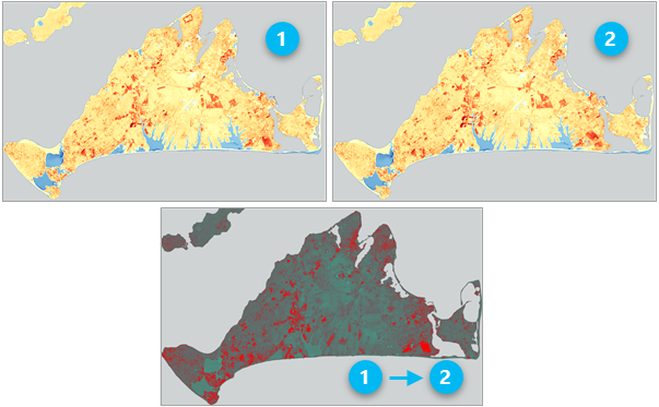
Pixel value change detection—ArcGIS AllSource

Change detection using continuous data is based on computing the differences between optical imagery or modeled data—such as temperature or wind speed—on a pixel-by-pixel basis.

The purpose of comparing continuous modeled data is typically to identify areas that have changed in magnitude or in a particular direction, usually over a period of time. ArcGIS AllSource provides several methods for comparing multiple continuous raster datasets.

Pixel value change detection between two vegetation index rasters

The Compute Change raster function computes the difference between two raster layers on the fly. Only the pixels within the visible extent are processed, and if zoomed out beyond the source resolution of the input data, the pixels are resampled to a larger size to speed up processing. This is a way to compute change for quick visualization and assessment of change. You can combine this function with other raster functions for a more complex workflow.

The Compute Change Raster geoprocessing tool computes the difference between two raster datasets and generates a new raster dataset containing the change information. You can combine this tool with other tools for a more complex workflow.

The Change Detection Wizard combines tools and functions to guide you through the process of performing categorical change detection, pixel value change detection, spectral change detection, or time series change detection. You can compare two raster datasets, or two slices in a multidimensional raster dataset.

The following section provides details on each pane in the Change Detection Wizard when performing continuous change detection.

Change Detection Wizard

The Change Detection Wizard is launched from the Change Detection drop-down button on the Imagery tab, in the Analysis group. The button is unavailable if you are not working in a 2D map scene, or if you do not have the Image Analyst extension.

Configure pane

The first pane in the Change Detection Wizard is the Configure pane, where you set the Change Detection Method value. To compare continuous datasets, set Change Detection Method to Pixel Value Change.

If a continuous raster is selected in the Contents pane when the wizard is launched, the Change Detection Method option is set to Pixel Value Change by default.


Parameter	Description
From Raster	The first raster to be used in the computation. To evaluate change from time 1 (earlier) to time 2 (later), enter the time 1 raster.
To Raster	The second raster to be used in the computation. To evaluate change from time 1 (earlier) to time 2 (later), enter the time 2 raster.

To compare two slices in a multidimensional dataset, enter the multidimensional raster as the From Raster parameter. The Configure pane updates with the parameters in the table below.


Parameter	Description
Variable	The variable to be analyzed.
Dimension	The dimension field to use to compare slices.
From Slice	The first slice to be used in the computation. To evaluate change from time 1 (earlier) to time 2 (later), enter the time 1 slice.
To Slice	The second slice to be used in the computation. To evaluate change from time 1 (earlier) to time 2 (later), enter the time 2 slice.
Processing Extent	The processing extent for the output.
X Skip Factor	The x skip factor used to calculate statistics and the histogram for the change raster.
Y Skip Factor	The y skip factor used to calculate statistics and the histogram for the change raster.

Band Difference pane

The Band Difference pane allows you to specify how to compare the input continuous raster datasets. If the data is multiband imagery, you can compare a single band between the two images or first calculate a band index before comparing.


Parameter	Description
Difference Type	The difference method to use in the calculation. Absolute—The mathematical difference, or subtraction, between the pixel values in the From Raster parameter and the pixel values in the To Raster parameter. `Output = (To Raster) - (From Raster)` This is the default. Relative—The difference in pixel values accounting for the quantities of the values being compared. `Output = (To Raster - From Raster) / max(To Raster, From Raster)`
Band Difference Method	Choose how you want to compare the continuous rasters. Single Band Difference—Calculate the difference between band values for a single band in each raster. Band Index Difference—Calculate a band index on each raster; then calculate the difference between index values.
From Raster Band and To Raster Band	Select the band in the From Raster parameter and the band in the To Raster parameter to compare in the calculation. This parameter is required when Band Difference Method is set to Single Band Difference. Typically, you compare pixel values from the same band in both images. For example, compare the Near Infrared band values between two dates. Occasionally, the band indexes are different between the two images, for example, if comparing Landsat 5 imagery to Landsat 8 imagery, so it is important to specify the band from each image.
Band Index	Select the band index to calculate for each raster before computing the difference between them. This parameter is required when Band Difference Method is set to Single Band Difference. The list of options is the same list of indexes available in the Indices Gallery. You need to specify the bands required to generate the index for each image.
Cell Size Type	Choose which cell size to use in the output raster. If all the input cell sizes are the same, all the options will yield the same results. First Of—Use the first cell size of the input rasters. Min Of—Use the smallest cell size of all the input rasters. Max Of—Use the largest cell size of all the input rasters. This is the default. Mean Of—Use the mean cell size of all the input rasters. Last Of—Use the last cell size of the input rasters.
Extent Type	Choose which extent should be used in the output raster: First Of—Use the extent of the first input raster to determine the processing extent. Intersection Of—Use the extent of the overlapping pixels to determine the processing extent. This is the default. Union Of—Use the extent of all the rasters to determine the processing extent. Last Of—Use the extent of the last input raster to determine the processing extent.

Click Preview to add a preview layer to the map, using the options you specified. You can modify the options and click Update Preview to refresh the preview layer with the new options.

Note:

The preview layers are generated using raster functions. When zoomed out beyond the source resolution, raster functions process the data using a resampled pixel size. To ensure the preview looks the way you want to see in your final result, zoom to the source resolution of the data. Right-click the preview layer and click Zoom to Source Resolution.

When you click Next in the Band Difference pane, the wizard computes the band index (if applicable), computes the difference between the rasters, and calculates the histogram of difference values. This may take some time depending on the size of your datasets.

Classify Difference pane

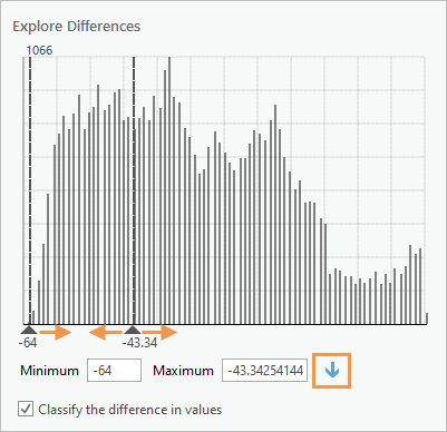
The Classify Difference pane allows you to explore the differences in pixel values on the fly in your map, and use the information to classify the results. For example, you can classify changes in NDVI into Loss or Gain classes, or you can classify differences in NIR band values to extract a burn scar, and classify it as a Burn Area class.

The Explore Differences section takes up the top half of the Classify Difference pane.

The Explore Differences section and interactive histogram

The histogram of difference values is displayed along with interactive handles for visualizing change. The Preview_Mask layer is added to the map by default when this pane is opened. When you drag the minimum and maximum histogram handles to different values in the histogram, the pixel values between the minimum and maximum are visible in the Preview_Mask layer on your map. All other pixel values are masked out and not visible. It may be easier to see the values if all other layers in the map are turned off. You can also modify the symbology of the Preview_Mask layer to more easily view the results.

To skip classification and retain the original pixel value differences, uncheck the Classify the difference in values parameter, and click Next to move on to the next pane.

Use the interactive histogram to generate classes

To use the interactive histogram to generate classes, complete the following steps:

Drag the minimum and maximum handles in the histogram until you have identified the change information that is important to your analysis (for example, strong negative change).
Click the Add New Class button .
The minimum and maximum values selected in the histogram are added as minimum and maximum class values in the Classify Output table at the bottom of the pane.
In the Classify Output table, add the class value (an integer) to the Output field and the name of the class to the Class Name field. These are required.
Specify the color to use to symbolize the class.

Manually generate classes

To manually enter class information, without using the interactive histogram, complete the following steps:

Click the Generate button .
In the Generate pane, set the Maximum Value parameter to the number of classes you want to generate.
You can specify a base name for the classes associated with each unique value. You can also specify the color scheme and the transparency for the class symbology.
When finished, click OK.
In the Classify Output table, manually type in the Minimum and Maximum difference field values for each class.

Click Preview to add a preview layer to the map, using the options you specified. You can modify the options and click Update Preview to refresh the preview layer with the new options.

Note:

Post-processing pane

The Post-processing pane allows you to smooth your results and generate an output.


Parameter	Description
Smoothing Neighborhood	The size of the focal neighborhood to use, in pixel rows and columns, to smooth your results. None—Do not perform smoothing. This is the default. 3 × 3—Smooth results based on a neighborhood of 3 pixel rows by 3 pixel columns. 5 × 5—Smooth results based on a neighborhood of 5 pixel rows by 5 pixel columns. 7 × 7—Smooth results based on a neighborhood of 7 pixel rows by 7 pixel columns.
Statistics Fill Method	The statistical method to use to recalculate pixel values for a smoother result. Minimum—Calculates the minimum value of the pixels within the neighborhood. Maximum—Calculates the maximum value of the pixels within the neighborhood. Mean—Calculates the average value of the pixels within the neighborhood. This is the default. Standard Deviation—Calculates the standard deviation value of the pixels within the neighborhood. Median—Calculates the median value of pixels within the neighborhood. Majority—Calculates the majority value, or the value that occurs most frequently, of the pixels within the neighborhood. Minority—Calculates the minority value, or the value that occurs least frequently, of the pixels within the neighborhood.
Save Result As	Specify the output type to generate. Raster Dataset—Results are saved as a raster dataset. Raster Function Template—Results are saved as a raster function template to be used for additional processing. Feature Class—Results are saved as a polygon feature class.
Output Dataset	The name of the output dataset. This parameter is only available if Save Result As is set to Raster Dataset or Feature Class. If the output is a raster dataset, specify the file extension to generate a raster in a supported format.

For additional smoothing options, you can use the Statistics raster function on your results. Choose None as the Smoothing Neighborhood in the wizard, and use the Statistics raster function on the output raster dataset.

Click Preview to add a preview layer to the map, using the options you specified. You can modify the options and click Update Preview to refresh the preview layer with the new options.

Note:

Example

The following example extracts loss in Soil Adjusted Vegetation Index (SAVI) values between two Landsat 8 images.

Add the two Landsat 8 images to your map.
With the earlier image layer selected in the Contents pane, launch the Change Detection Wizard from the Imagery tab in the Analysis group.
In the Configure pane, the From Raster parameter is set to the earlier raster layer.
Set the To Raster parameter to the later raster layer.
Click Next.
In the Band Difference pane, set the analysis to compute changes in SAVI values.
1. Set the Difference Type parameter to Absolute.
2. Set the Band Difference Method parameter to Band Index Difference.
3. In the Band Index Parameters — From Raster section, set Near Infrared Band Index to Band 5 and set Red Band Index to Band 4. Keep the default Soil-brightness correction factor value of 0.5.
4. In the Band Index Parameters — To Raster section, set Near Infrared Band Index to Band 5 and set Red Band Index to Band 4. Keep the default Soil-brightness correction factor value of 0.5.
5. Set the Cell Size Type parameter to Max of, and the Extent Type parameter to Intersection of.
Click Next.
In the Classify Difference pane, drag the maximum histogram handle to 0, and leave the minimum histogram handle at the lowest negative value. Click Add New Class.
In the Classify Output table, set the Output field value to 1, the Class Name field to Loss, and use the color picker to select a red color.
Click Next.
In the Post-processing pane, set the Smoothing Neighborhood parameter to 3 x 3 and the Statistics Fill Method parameter to Majority.
For the Output Dataset parameter, type SAVI_Loss.tif. Click Run.
When the dataset is added to the map, click Finish to close the Change Detection Wizard.

Feedback on this topic?