Available with Image Analyst license.
The following concepts and methods are key for understanding and performing pixel classification in AllSource.
Semantic segmentation
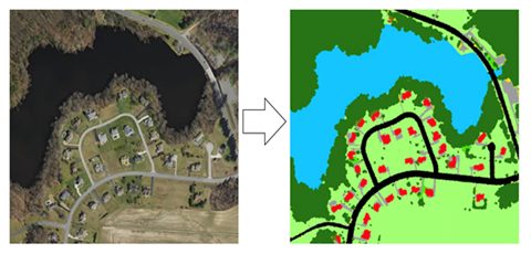
Semantic segmentation, also known as pixel-based classification, is an important task where classification of each pixel belongs to a particular class. In GIS, you can use segmentation for land cover classification or for extracting roads or buildings from satellite imagery.

The goal of semantic segmentation is the same as traditional image classification in remote sensing. This is usually conducted by applying traditional machine learning techniques, such as random forest or maximum likelihood classifier. Like image classification, there are also two inputs for semantic segmentation:
- A raster image that contains multiple bands
- A label image that contains the label for each pixel
Training with sparse data
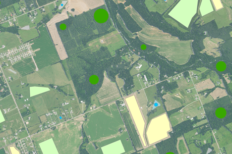
Not every pixel in an image is used in the classification of training samples. This is known as sparse training samples. Below is a diagram of the image and sparse training samples being selected. In this case of sparse training samples as below, you must set the ignore class parameter to 0. This will ignore the pixels that have not been classified for training.

U-Net
U-Net architecture can be thought of as an encoder network followed by a decoder network. Semantic segmentation classifies features of pixels, and this pixel level classification is learned at different stages of the encoder.
The encoder is the first half of the U-Net process. The encoder is usually a pretrained classification network such as VGG or ResNet, where you apply convolution blocks followed by a maxpool downsampling to encode the input image into feature representations at multiple levels1. The decoder is the second half of the process. The goal is to semantically project the discriminative features (lower resolution) learned by the encoder onto the pixel space (higher resolution) to get a dense classification. The decoder consists of upsampling and concatenation followed by regular convolution operations1
References
[1] Olaf Ronneberger, Philipp Fischer, Thomas Brox. U-Net: Convolutional Networks for Biomedical Image Segmentation, https://arxiv.org/abs/1505.04597, (2015).
PSPNet
The Pyramid Scheme Parsing Network (PSPNet) model consists of an encoder and a decoder. The encoder is responsible for the extracting features from the image. The decoder predicts the class of the pixel at the end of the process.
Deep Lab
Fully Convolutional Neural Networks (FCNs) are often used for semantic segmentation. One challenge with using FCNs on images for segmentation tasks is that input feature maps become smaller while traversing through the convolutional and pooling layers of the network. This causes loss of information about the images and results in an output where predictions are of low resolution and the object boundaries are fuzzy.
The DeepLab model addresses this challenge by using Atrous convolutions and Atrous Spatial Pyramid Pooling (ASPP) modules. The first version of DeepLab (DeepLabV1) Uses Atrous Convolution and Fully Connected Conditional Random Field (CRF) to control the resolution at which image features are computed.
AllSource uses DeepLabV3. DeepLabV3 also uses Atrous Convolution, however it also uses an improved ASPP module by including batch normalization and image-level features. It no longer uses the obsolete CRF (Conditional Random Field), as used in V1 and V2.
The DeepLabV3 model has the following architecture:
- Features are extracted from the backbone network, such as VGG, DenseNet, and ResNet.
- To control the size of the feature map, Atrous convolution is used in the last few blocks of the backbone.
- On top of extracted features from the backbone, an ASPP network is added to classify each pixel corresponding to their classes.
- The output from the ASPP network is passed through a 1 by 1 convolution to get the actual size of the image, which will be the final segmented mask for the image.